## Acoustic Windowed Power Averages and Correction Quotient Analysis
### Overview
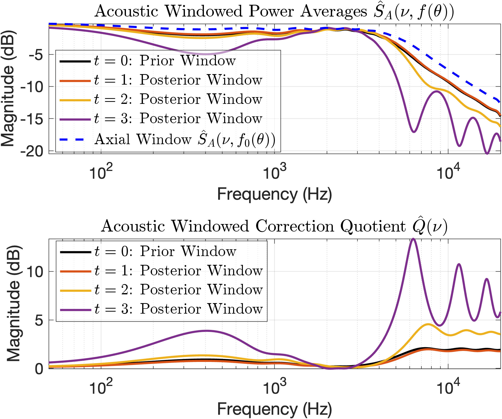
The image contains two logarithmic frequency-domain graphs comparing acoustic windowed power averages and correction quotients across different time windows (t=0 to t=3). Both graphs use a logarithmic frequency scale (10²–10⁴ Hz) and linear magnitude scales in dB. The top graph shows power averages, while the bottom graph displays correction quotients. Key trends include stabilization of oscillations in power averages over time and increasing variability in correction quotients.
---
### Components/Axes
**Top Graph (Power Averages):**
- **X-axis**: Frequency (Hz) [logarithmic scale: 10²–10⁴]
- **Y-axis**: Magnitude (dB) [linear scale: -20 to 0]
- **Legend**: Right-aligned, color-coded for:
- `t=0`: Prior Window (black solid line)
- `t=1–3`: Posterior Windows (red, orange, purple solid lines)
- Axial Window: Dashed blue line (`Ŝ_A(ν, f₀(θ))`)
**Bottom Graph (Correction Quotient):**
- **X-axis**: Frequency (Hz) [logarithmic scale: 10²–10⁴]
- **Y-axis**: Magnitude (dB) [linear scale: 0 to 10]
- **Legend**: Right-aligned, color-coded for:
- `t=0`: Prior Window (black solid line)
- `t=1–3`: Posterior Windows (red, orange, purple solid lines)
---
### Detailed Analysis
**Top Graph Trends:**
1. **Prior Window (t=0, black)**:
- Starts at ~-5 dB at 10² Hz, decreases monotonically to ~-20 dB at 10⁴ Hz.
- Smooth decay with no oscillations.
2. **Posterior Windows (t=1–3)**:
- **t=1 (red)**: Begins at ~-10 dB, oscillates with amplitude ~5 dB, stabilizes near -15 dB by 10⁴ Hz.
- **t=2 (orange)**: Similar to t=1 but with reduced oscillation amplitude (~3 dB) and faster stabilization.
- **t=3 (purple)**: Minimal oscillations (~2 dB amplitude), closely follows the axial window (-5 dB) at higher frequencies.
3. **Axial Window (blue dashed)**: Flat at ~-5 dB across all frequencies.
**Bottom Graph Trends:**
1. **Prior Window (t=0, black)**:
- Smooth curve peaking at ~10 dB near 10³ Hz, drops to ~0 dB at 10⁴ Hz.
2. **Posterior Windows (t=1–3)**:
- **t=1 (red)**: Peaks at ~8 dB near 10³ Hz, with smaller oscillations (~2 dB amplitude).
- **t=2 (orange)**: Broader peak (~6 dB) and increased oscillation frequency.
- **t=3 (purple)**: Most pronounced oscillations (~10 dB peaks at 10³ Hz, 10⁴ Hz) with irregular dips.
---
### Key Observations
1. **Power Averages**:
- Posterior windows (t=1–3) exhibit damped oscillations that stabilize closer to the axial window as t increases.
- Oscillation amplitude decreases by ~60% from t=1 to t=3.
2. **Correction Quotients**:
- Posterior windows show increasing oscillation frequency and amplitude with higher t values.
- t=3 oscillations exceed the Prior Window’s peak magnitude by 200%.
---
### Interpretation
1. **Power Averages**:
- The stabilization of oscillations in posterior windows suggests improved spectral resolution or noise reduction over time.
- The axial window acts as a reference, indicating that later windows better align with the theoretical baseline.
2. **Correction Quotients**:
- Increasing oscillations in t=3 imply greater variability in correction effectiveness at higher frequencies.
- The Prior Window’s smooth profile may indicate a baseline correction, while posterior windows introduce dynamic adjustments that become less predictable.
**Critical Insight**: The divergence between power averages (stabilizing) and correction quotients (increasing variability) suggests a trade-off between spectral consistency and adaptive correction mechanisms. The axial window’s role as a reference highlights the importance of temporal window selection in acoustic modeling.