\n
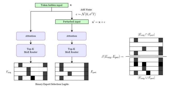
## Diagram: Mixture of Experts (MoE) with Noise Injection
### Overview
This diagram illustrates a process for injecting noise into a Mixture of Experts (MoE) model. The core idea is to perturb the input and then compare the expert selections made on the original and perturbed inputs to calculate a loss function. The diagram shows the flow of data through attention layers, MoE routers, and the resulting expert selections.
### Components/Axes
The diagram consists of the following components:
* **Token hidden input (x):** The initial input to the system.
* **Add Noise:** A process that adds noise, denoted as ε ~ N(0, σ²I), to the input.
* **Perturbed input (x'):** The input after noise has been added (x' = x + ε).
* **Attention Layers:** Two parallel attention layers processing the original and perturbed inputs.
* **Top-K MoE Router:** Two parallel MoE routers, one for each attention layer output.
* **Eorig:** Represents the expert selection based on the original input. Displayed as a grid with black and white cells.
* **Epert:** Represents the expert selection based on the perturbed input. Displayed as a grid with black and white cells.
* **J(Eorig, Epert):** A loss function that compares the expert selections.
* **Eorig ∩ Epert:** The intersection of the experts selected for the original and perturbed inputs. Displayed as a grid with black and white cells.
* **Eorig ∪ Epert:** The union of the experts selected for the original and perturbed inputs. Displayed as a grid with black and white cells.
* **Binary Expert Selection Logits:** Label for the grids representing Eorig and Epert.
### Detailed Analysis / Content Details
The diagram shows a parallel processing structure. The original input 'x' and the perturbed input 'x'' both pass through an attention layer and then a Top-K MoE router. The outputs of the routers, Eorig and Epert, are represented as grids. Each grid appears to be 4x4, with some cells colored black and others white. The black cells likely represent the experts that were selected for that input.
The intersection (Eorig ∩ Epert) and union (Eorig ∪ Epert) of the expert selections are also shown as grids, again 4x4. The intersection shows which experts were selected by both the original and perturbed inputs, while the union shows all experts selected by either input.
The noise added is defined as ε ~ N(0, σ²I), indicating a Gaussian distribution with a mean of 0 and a variance of σ²I, where I is the identity matrix.
The grids representing Eorig, Epert, Eorig ∩ Epert, and Eorig ∪ Epert all have the same structure. The black and white cells are arranged in a pattern.
* **Eorig:** The top two rows are entirely black, the third row has the first two cells black, and the last row has the last two cells black.
* **Epert:** The top row has the first two cells black, the second row is entirely black, the third row has the last two cells black, and the last row is entirely black.
* **Eorig ∩ Epert:** The first two cells of the second row are black, and the last two cells of the third row are black.
* **Eorig ∪ Epert:** The first two cells of the first row are black, the second and third rows are entirely black, and the last two cells of the last row are black.
### Key Observations
The diagram highlights the comparison of expert selections under noise injection. The loss function J(Eorig, Epert) is likely designed to penalize significant differences between the expert selections made on the original and perturbed inputs. This suggests a regularization technique to improve the robustness of the MoE model. The grids show a clear difference between the expert selections for the original and perturbed inputs, indicating that the noise does indeed influence the router's decisions.
### Interpretation
This diagram demonstrates a method for regularizing a Mixture of Experts model by injecting noise into the input. The core idea is to encourage the model to make consistent expert selections even when the input is slightly perturbed. By comparing the expert selections on the original and perturbed inputs, the loss function J(Eorig, Epert) can identify and penalize unstable router behavior. This approach can improve the model's generalization ability and robustness to adversarial attacks. The use of the intersection and union of expert selections provides a way to quantify the degree of overlap and difference between the two sets of experts, which is then used to calculate the loss. The Gaussian noise distribution is a common choice for adding small, random perturbations to the input. The diagram provides a visual representation of the process, making it easier to understand the underlying principles of this regularization technique. The grids are a visual representation of the binary expert selection logits, showing which experts are activated for each input.