## Diagram: Grid to Data Structure Transformation
### Overview
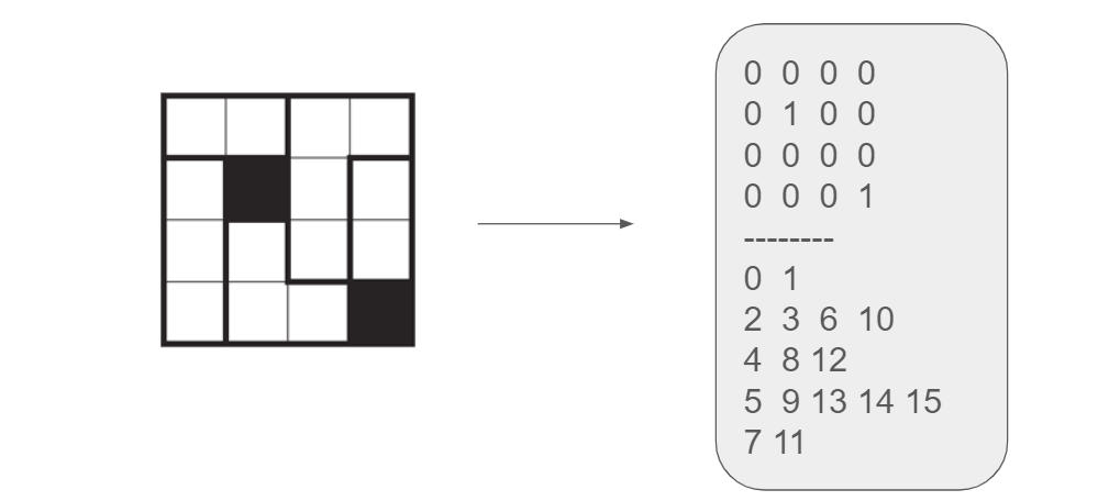
The image displays a two-part diagram illustrating a transformation from a visual grid representation to a structured numerical data format. On the left is a 4x4 grid with specific cells filled in black. An arrow points to the right, leading to a rounded rectangular container holding two distinct sets of numerical data separated by a dashed line. The diagram visually explains how a spatial or binary pattern is encoded into a hierarchical or indexed data structure.
### Components/Axes
1. **Left Component (Source Grid):**
* A 4x4 grid with uneven internal borders, creating a non-uniform cell structure.
* Two cells are filled with solid black.
* **Black Cell Positions (approximate):** Row 2, Column 2 and Row 4, Column 4 (assuming 1-based indexing from top-left).
2. **Transformation Indicator:**
* A simple right-pointing arrow (`→`) connects the left grid to the right data container, indicating a mapping or conversion process.
3. **Right Component (Data Container):**
* A light gray, rounded rectangle containing text.
* The content is divided into two sections by a horizontal dashed line (`---------`).
* **Top Section (Binary Matrix):** A 4x4 matrix of binary digits (0s and 1s).
* **Bottom Section (Indexed Lists):** Five rows of integers, with a varying number of entries per row.
### Detailed Analysis
**Top Section - Binary Matrix Transcription:**
```
0 0 0 0
0 1 0 0
0 0 0 0
0 0 0 1
```
* **Trend/Pattern:** This matrix is a direct binary representation of the left grid. A '1' corresponds to a black cell, and a '0' corresponds to a white cell. The '1's are located at positions (2,2) and (4,4), perfectly matching the visual grid.
**Bottom Section - Indexed Lists Transcription:**
```
0 1
2 3 6 10
4 8 12
5 9 13 14 15
7 11
```
* **Content:** This section contains the integers from 0 to 15, partitioned into five groups.
* **Spatial Grounding:** The numbers are arranged in a left-aligned list format within the container, below the dashed line.
* **Observation:** The grouping does not follow a simple sequential order. The numbers 5 and 15 (which correspond to the positions of the '1's in the binary matrix if cells are numbered 0-15 in row-major order) appear together in the fourth row of this list.
### Key Observations
1. **Direct Mapping:** The top numerical section is an exact binary encoding of the visual grid pattern.
2. **Non-Sequential Grouping:** The bottom section's grouping of numbers (0-15) is not sequential, suggesting it represents a specific traversal order, hierarchical decomposition (like a quadtree), or clustering based on the grid's structure.
3. **Structural Emphasis:** The thicker borders in the left grid may indicate a hierarchical subdivision (e.g., dividing the 4x4 grid into four 2x2 quadrants), which could be related to the grouping logic in the bottom list.
### Interpretation
This diagram demonstrates a method for converting a 2D spatial pattern (the grid) into a compact, structured data representation. The process involves two key steps:
1. **Binary Encoding:** First, the visual pattern is translated into a standard binary matrix, which is a fundamental format for digital image representation and processing.
2. **Structural Indexing:** Second, the cells of the grid are assigned unique indices (0-15) and then grouped into a specific, non-sequential order. This grouping likely reflects an underlying **spatial indexing scheme** or **hierarchical data structure**. Common examples include:
* **Quadtree Decomposition:** The grid is recursively divided into quadrants. The list order might represent a depth-first traversal of the quadtree nodes.
* **Space-Filling Curve (e.g., Z-order/Morton order):** The indices follow a path that preserves spatial locality, which is useful for efficient range queries in databases or image compression.
* **Run-Length Encoding (RLE) Variant:** The groups could represent runs of similar cells (e.g., background vs. foreground), though the presence of all numbers 0-15 makes this less likely.
**The core purpose** of the diagram is to illustrate how spatial information is abstracted and organized for computational efficiency. The black cells (data points of interest) are embedded within a larger structure, and the bottom list shows how all elements of that structure are cataloged in a specific, meaningful order that likely optimizes for operations like searching, compression, or spatial analysis. The transformation moves from a human-visual format to a machine-optimized format.