\n
## Chart: Convergence of Log Probability Ratio
### Overview
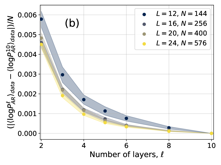
The image presents a line chart illustrating the convergence of the log probability ratio as a function of the number of layers. The chart displays four data series, each representing a different system size, with shaded regions indicating the uncertainty or variance around each line. The y-axis represents the average log probability ratio difference, normalized by the system size (N), while the x-axis represents the number of layers (l).
### Components/Axes
* **Title:** (b) - likely a sub-figure identifier.
* **X-axis Label:** Number of layers, *l* (ranging from approximately 2 to 10).
* **Y-axis Label:** ⟨(log *P*<sub>*AR*</sub><sup>*l*</sup><sub>data</sub> - (log *P*<sub>*AR*</sub><sup>10</sup><sub>data</sub>))/N⟩ (ranging from approximately 0.000 to 0.006).
* **Legend:** Located in the top-right corner.
* Dark Blue: L = 12, N = 144
* Gray: L = 16, N = 256
* Light Gray: L = 20, N = 400
* Yellow: L = 24, N = 576
* **Data Series:** Four lines representing different system sizes (L and N values).
* **Shaded Regions:** Lightly shaded areas around each line, representing the uncertainty or standard deviation.
* **Gridlines:** Vertical gridlines are present to aid in reading values on the x-axis.
### Detailed Analysis
The chart shows a clear downward trend for all data series. As the number of layers (*l*) increases, the average log probability ratio difference decreases, indicating convergence.
* **L = 12, N = 144 (Dark Blue):**
* At *l* = 2, the value is approximately 0.0058.
* At *l* = 4, the value is approximately 0.0035.
* At *l* = 6, the value is approximately 0.0018.
* At *l* = 8, the value is approximately 0.0008.
* At *l* = 10, the value is approximately 0.0002.
* **L = 16, N = 256 (Gray):**
* At *l* = 2, the value is approximately 0.0055.
* At *l* = 4, the value is approximately 0.0032.
* At *l* = 6, the value is approximately 0.0016.
* At *l* = 8, the value is approximately 0.0007.
* At *l* = 10, the value is approximately 0.0002.
* **L = 20, N = 400 (Light Gray):**
* At *l* = 2, the value is approximately 0.0052.
* At *l* = 4, the value is approximately 0.0030.
* At *l* = 6, the value is approximately 0.0015.
* At *l* = 8, the value is approximately 0.0006.
* At *l* = 10, the value is approximately 0.0001.
* **L = 24, N = 576 (Yellow):**
* At *l* = 2, the value is approximately 0.0050.
* At *l* = 4, the value is approximately 0.0028.
* At *l* = 6, the value is approximately 0.0014.
* At *l* = 8, the value is approximately 0.0005.
* At *l* = 10, the value is approximately 0.0001.
The shaded regions around each line indicate some variability in the data, but the overall trend remains consistent across all system sizes. The lines appear to converge towards a value close to zero as the number of layers increases.
### Key Observations
* All data series exhibit a similar downward trend, suggesting that the convergence behavior is independent of the system size (within the range tested).
* The convergence appears to be faster initially (between *l* = 2 and *l* = 6) and then slows down as the number of layers increases.
* The values for larger system sizes (L=24, N=576) are consistently slightly lower than those for smaller system sizes, although the difference is small.
### Interpretation
This chart demonstrates the convergence of a certain property (represented by the log probability ratio) as the number of layers in a system increases. The convergence suggests that the system is approaching a stable state or equilibrium. The normalization by the system size (N) indicates that the convergence rate is independent of the absolute size of the system. The shaded regions represent the uncertainty in the measurements, which could be due to statistical fluctuations or other sources of noise. The fact that all lines converge to approximately zero suggests that the property being measured becomes negligible as the number of layers increases. This could be indicative of a well-behaved system that reaches a stable configuration with sufficient layers. The consistent trend across different system sizes suggests that the observed behavior is a general property of the system and not an artifact of a specific size.