## Line Graph: Layer-wise Autoregressive Probability Metric
### Overview
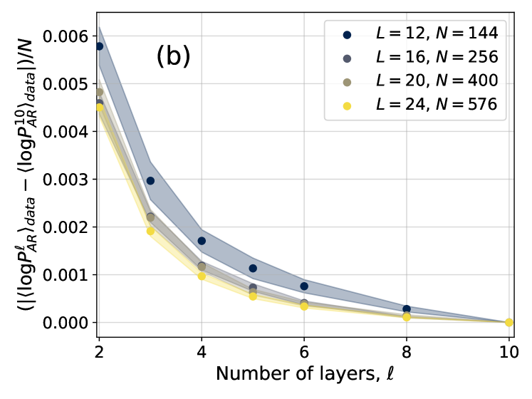
The image is a scientific line graph labeled "(b)" in the top-left corner of the plot area. It displays the relationship between the number of layers (ℓ) in a model and a normalized, absolute difference metric involving autoregressive probabilities. The graph contains four data series, each corresponding to a different model configuration defined by parameters L and N. All series show a decreasing trend as the number of layers increases.
### Components/Axes
* **X-Axis:** Labeled "Number of layers, ℓ". The axis has major tick marks at values 2, 4, 6, 8, and 10.
* **Y-Axis:** Labeled with the complex mathematical expression: `( |⟨log P_AR^ℓ⟩_data - ⟨log P_AR^10⟩_data| ) / N`. The axis scale ranges from 0.000 to 0.006, with major tick marks at intervals of 0.001.
* **Legend:** Positioned in the top-right corner of the plot area. It defines four data series:
* Dark Blue Circle: `L = 12, N = 144`
* Gray Circle: `L = 16, N = 256`
* Tan/Brown Circle: `L = 20, N = 400`
* Yellow Circle: `L = 24, N = 576`
* **Data Series:** Each series is represented by a line connecting circular markers. A shaded region of the corresponding color surrounds each line, likely indicating a confidence interval or standard deviation.
### Detailed Analysis
The graph plots the value of the y-axis metric against the number of layers (ℓ) for four model configurations. The data points are at ℓ = 2, 4, 6, 8, and 10.
**Trend Verification:** All four lines exhibit a clear, monotonic downward slope from left to right. The rate of decrease is steepest between ℓ=2 and ℓ=4, and the curves flatten as ℓ increases, converging near zero at ℓ=10.
**Approximate Data Points (Visual Estimation):**
| ℓ (Layers) | L=12, N=144 (Dark Blue) | L=16, N=256 (Gray) | L=20, N=400 (Tan) | L=24, N=576 (Yellow) |
| :--- | :--- | :--- | :--- | :--- |
| **2** | ~0.0058 | ~0.0050 | ~0.0048 | ~0.0045 |
| **4** | ~0.0017 | ~0.0012 | ~0.0011 | ~0.0010 |
| **6** | ~0.0008 | ~0.0005 | ~0.0004 | ~0.00035 |
| **8** | ~0.0003 | ~0.0002 | ~0.00015 | ~0.0001 |
| **10** | ~0.0000 | ~0.0000 | ~0.0000 | ~0.0000 |
**Spatial Grounding & Component Isolation:**
* **Header Region:** Contains the label "(b)" in the top-left.
* **Main Chart Region:** The plot area. The legend is anchored in the top-right. The data lines originate from the top-left (high y-value at low ℓ) and converge at the bottom-right (y≈0 at ℓ=10).
* **Footer Region:** Contains the x-axis label.
### Key Observations
1. **Consistent Hierarchy:** At every layer count (ℓ) before convergence, the series maintain a strict order from highest to lowest y-value: `L=12, N=144` > `L=16, N=256` > `L=20, N=400` > `L=24, N=576`.
2. **Convergence:** All data series converge to a value of approximately 0.000 at ℓ=10. This is expected, as the y-axis metric measures the difference from the value at ℓ=10 (`⟨log P_AR^10⟩_data`).
3. **Diminishing Returns:** The most significant reduction in the metric occurs within the first few layers (ℓ=2 to ℓ=4). Subsequent layers yield progressively smaller decreases.
4. **Model Size Correlation:** Larger models (higher L and N) start with a lower initial value of the metric at ℓ=2 and maintain lower values throughout, though the absolute difference between series diminishes as ℓ increases.
### Interpretation
This graph likely analyzes the internal probability distributions of autoregressive models of varying depths and widths. The y-axis metric quantifies how much the model's probability distribution at a given layer ℓ differs from its final distribution at layer 10, normalized by the parameter N.
The data suggests two key insights:
1. **Layer-wise Refinement:** The model's internal representation, as measured by this probability metric, undergoes the most dramatic change in the early layers. This implies that the foundational features or predictions are established quickly, with later layers performing finer adjustments.
2. **Impact of Model Scale:** Larger models (higher L and N) appear to have a "head start" – their internal distributions at early layers are already closer to their final state (lower y-value). This could indicate that increased model capacity allows for more efficient or stable internal processing from the outset.
The convergence at ℓ=10 is a mathematical certainty by the definition of the metric, serving as a sanity check for the plot. The consistent ordering of the lines provides strong evidence that model scale (both depth L and width N) systematically influences the trajectory of this internal refinement process. The shaded regions, while not quantified, suggest the variance or uncertainty in this metric is also larger for smaller models and in the early layers.