## 3D Surface Plot: Minimised Energy vs. Theta 1 and Theta 2 ### Overview The image is a 3D surface plot visualizing the relationship between "Minimised Energy" and two variables, theta1 (θ₁) and theta2 (θ₂). The surface is colored based on the energy level, with lower energy values represented by purple/blue and higher energy values represented by yellow/green. The plot shows two distinct minima and a central peak. ### Components/Axes * **X-axis (θ₁):** Ranges from approximately -5 to 5. * **Y-axis (θ₂):** Ranges from approximately -5 to 5. * **Z-axis (Minimised Energy):** Ranges from -7 to -1. * **Color Gradient:** Represents the magnitude of the "Minimised Energy," with purple/blue indicating lower values and yellow/green indicating higher values. ### Detailed Analysis The surface plot exhibits the following key features: * **Two Minima:** There are two distinct low-energy regions (purple/blue) located symmetrically with respect to the θ₂ axis. One is located at approximately θ₁ = -4, θ₂ = 4, and the other at θ₁ = -4, θ₂ = -4. The energy at these minima is approximately -7. * **Central Peak:** A high-energy region (yellow/green) is located near θ₁ = 0, θ₂ = 0. The energy at this peak is approximately -1. * **Symmetry:** The surface appears to be roughly symmetrical with respect to the θ₂ axis. * **Slopes:** The surface slopes steeply upwards from the minima towards the central peak. ### Key Observations * The global minima of the "Minimised Energy" occur at two distinct points in the θ₁-θ₂ space. * The energy landscape is characterized by steep gradients, suggesting a strong dependence of the energy on the values of θ₁ and θ₂. * The symmetry of the plot suggests that the energy function might have some inherent symmetry properties. ### Interpretation The 3D surface plot visualizes an energy landscape where the "Minimised Energy" depends on two parameters, θ₁ and θ₂. The presence of two distinct minima suggests that there are two stable configurations or solutions for the system being modeled. The central peak represents an unstable configuration or a barrier between the two stable states. The steep slopes indicate that small changes in θ₁ or θ₂ can lead to significant changes in the energy. This type of plot is commonly used in optimization problems to visualize the objective function and identify potential solutions.

\n ## 3D Surface Plot: Minimized Energy Landscape ### Overview The image depicts a 3D surface plot representing a minimized energy landscape. The plot visualizes the relationship between two parameters, θ₁ and θ₂, and their corresponding minimized energy value. The surface is colored to indicate energy levels, with warmer colors (yellow/orange) representing lower energy and cooler colors (green/purple) representing higher energy. ### Components/Axes * **X-axis:** θ₂ - ranges approximately from -4 to 4. * **Y-axis:** θ₁ - ranges approximately from -4 to 4. * **Z-axis:** Minimized Energy - ranges approximately from -7 to 1. * **Surface:** Represents the minimized energy value for different combinations of θ₁ and θ₂. * **Color Gradient:** Indicates energy levels. Yellow/orange represents lower energy, transitioning through green to purple for higher energy. ### Detailed Analysis The surface exhibits a complex shape with multiple local minima and a prominent central peak. * **Central Peak:** Located around θ₁ = 0 and θ₂ = 0, the surface rises to a local maximum with an energy value of approximately 1. * **Left Minimum:** A broad minimum extends from approximately θ₁ = -4 to θ₁ = 0 and θ₂ = -4, with energy values ranging from approximately -3 to -7. The minimum appears to be shallowest at θ₂ = -4. * **Right Minimum:** A similar broad minimum extends from approximately θ₁ = 0 to θ₁ = 4 and θ₂ = 4, with energy values ranging from approximately -3 to -7. The minimum appears to be shallowest at θ₂ = 4. * **Saddle Points:** There are saddle points visible where the surface changes curvature, indicating transitions between different energy minima. These are located around θ₁ = -2, θ₂ = 2 and θ₁ = 2, θ₂ = -2. * **Trend:** The surface generally decreases in energy as θ₁ and θ₂ move away from the central peak towards the minima on the left and right. ### Key Observations * The energy landscape is not symmetrical. The minima on the left and right sides of the plot are not identical in shape or depth. * The presence of multiple local minima suggests the possibility of multiple stable states or configurations. * The central peak represents an unstable state, as any small perturbation would likely cause the system to move towards one of the minima. ### Interpretation This plot likely represents the energy landscape of a system with two degrees of freedom, parameterized by θ₁ and θ₂. The minimized energy indicates the stability of different configurations of the system. The multiple minima suggest that the system can exist in several stable states, and the energy barrier between these states (represented by the height of the saddle points) determines the ease with which the system can transition between them. The shape of the landscape suggests a complex interplay between the two parameters, and the asymmetry indicates that the system is not invariant under certain transformations. This type of plot is common in fields like physics, chemistry, and machine learning, where it is used to visualize the energy landscape of a system and understand its behavior. The data suggests that the system will tend to settle into one of the two minima, and the specific minimum it settles into will depend on its initial conditions.

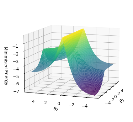
## 3D Surface Plot: Minimised Energy Landscape ### Overview The image displays a three-dimensional surface plot visualizing a function of two variables, θ₁ and θ₂. The plot illustrates how a quantity labeled "Minimised Energy" varies across a two-dimensional parameter space. The surface is rendered with a color gradient that maps directly to the energy value, providing an intuitive visual cue for the function's topography. ### Components/Axes * **Chart Type:** 3D Surface Plot. * **Axes:** * **X-axis (Foreground, Left-Right):** Labeled **θ₂**. The axis spans from approximately **-4** to **+4**, with major tick marks at intervals of 2 (-4, -2, 0, 2, 4). * **Y-axis (Depth, Front-Back):** Labeled **θ₁**. The axis spans from approximately **-4** to **+4**, with major tick marks at intervals of 2 (-4, -2, 0, 2, 4). * **Z-axis (Vertical):** Labeled **Minimised Energy**. The axis spans from **-7** to **-1**, with major tick marks at intervals of 1 (-7, -6, -5, -4, -3, -2, -1). * **Legend/Color Mapping:** There is no separate legend box. The surface itself uses a continuous color gradient to represent the Z-axis (Minimised Energy) value. The gradient transitions from **dark blue/purple** at the lowest energy values (near -7) through **teal/green** at intermediate values, to **bright yellow** at the highest energy values (near -1). ### Detailed Analysis * **Surface Topology:** The surface exhibits a complex, saddle-like shape with distinct features: * A prominent **peak** (local maximum) is located in the quadrant where both θ₁ and θ₂ are positive. The peak's apex is colored bright yellow, indicating the highest minimised energy value on the plot, approximately **-1.5 to -1.0**. * A deep **valley** (global minimum within the visible range) is located in the quadrant where θ₁ is negative and θ₂ is positive. This region is colored dark blue/purple, indicating the lowest energy value, approximately **-7.0**. * The surface slopes downward from the peak towards this valley and also towards the edges of the parameter space. * **Trend Verification:** * Moving from the valley (θ₁ ≈ -2, θ₂ ≈ +2) towards the peak (θ₁ ≈ +2, θ₂ ≈ +2), the surface slopes **steeply upward**, with the color shifting from dark blue to yellow. * Moving along the θ₂ axis at a fixed, positive θ₁ (e.g., θ₁ ≈ +2), the energy first increases to a ridge and then decreases, forming a curved "hill." * Moving along the θ₁ axis at a fixed, negative θ₂ (e.g., θ₂ ≈ -2), the energy shows a more gradual, undulating change. * **Spatial Grounding:** The vertical Z-axis is positioned on the left side of the plot. The θ₂ axis runs along the bottom front edge, and the θ₁ axis recedes into the depth on the right side. The highest point (yellow peak) is in the upper-right quadrant of the 3D space. The lowest point (dark blue valley) is in the lower-right quadrant. ### Key Observations 1. **Non-Convex Landscape:** The energy function is clearly non-convex, featuring at least one significant local maximum (the peak) and one deep global minimum (the valley) within the plotted domain. 2. **Parameter Sensitivity:** The energy is highly sensitive to changes in both θ₁ and θ₂, as evidenced by the steep gradients (sharp color changes) on the surface, particularly around the peak and leading into the valley. 3. **Asymmetric Features:** The landscape is not symmetric. The valley is deeper and more pronounced than any other depression, and the peak is a singular, sharp feature. ### Interpretation This plot likely represents the **loss or energy landscape** of a machine learning model or a physical system, where θ₁ and θ₂ are two parameters (e.g., weights in a neural network, coordinates in a physical system). The "Minimised Energy" is the objective function being optimized. * **The Goal:** In optimization contexts, the goal is typically to find the parameter set (θ₁, θ₂) that **minimizes** this energy. The deep blue valley represents the optimal (or a highly favorable) solution region. * **The Challenge:** The presence of the prominent yellow peak illustrates a significant **local maximum** or a region of high loss. An optimization algorithm starting near this peak could get stuck or have difficulty navigating towards the global minimum in the valley, highlighting a potential challenge for gradient-based methods. * **Relationship Between Parameters:** The curved, interconnected shape of the surface shows that the effect of changing θ₁ on the energy depends strongly on the current value of θ₂, and vice-versa. They are **interdependent parameters** in this system. * **Notable Anomaly:** The most striking feature is the sharp, isolated peak. In a typical loss landscape for well-behaved problems, one might expect smoother transitions or multiple similar minima. This pronounced maximum could indicate a specific, unstable configuration of the parameters that is highly undesirable. **In summary, the image provides a visual map of a complex optimization problem, revealing a challenging landscape with a clear target (the deep minimum) and a significant obstacle (the high peak) that an optimization process must navigate.**

## 3D Surface Plot: Minimised Energy Landscape ### Overview The image depicts a 3D surface plot visualizing a mathematical function's energy landscape. The plot features a color gradient from purple (lowest energy) to yellow (highest energy), with a grid overlay and labeled axes. The surface exhibits multiple peaks, troughs, and saddle points, suggesting a complex optimization problem or physical system. ### Components/Axes - **X-axis (θ₂)**: Ranges from -4 to 4, labeled with integer markers at -4, -2, 0, 2, 4. - **Y-axis (θ₁)**: Ranges from -4 to 4, labeled with integer markers at -4, -2, 0, 2, 4. - **Z-axis (Minimised Energy)**: Ranges from -7 to -1, with markers at -1, -2, -3, -4, -5, -6, -7. - **Grid**: Fine grid lines span all three axes, with darker lines at axis intersections. - **Color Gradient**: Smooth transition from purple (low energy) to yellow (high energy), with no explicit legend but implied by color intensity. ### Detailed Analysis 1. **Peaks**: - **Highest Peak**: Located at approximately (θ₂=0, θ₁=2), with energy ≈ -1 (yellow region). - **Secondary Peak**: Near (θ₂=2, θ₁=0), energy ≈ -2 (green-yellow transition). 2. **Troughs**: - **Deepest Trough**: At (θ₂=-4, θ₁=-4), energy ≈ -7 (dark purple). - **Secondary Trough**: Near (θ₂=4, θ₁=4), energy ≈ -6 (dark purple). 3. **Saddle Point**: - Located at (θ₂=0, θ₁=0), energy ≈ -3 (green region), acting as a critical point between peaks and troughs. 4. **Symmetry**: - The plot exhibits approximate symmetry about θ₂=0, with mirrored energy distributions in the θ₁ direction. ### Key Observations - The energy landscape is non-convex, with multiple local minima and maxima. - The deepest energy minimum (-7) occurs at the extreme corner (-4, -4), while the shallowest (-1) is near the origin. - The saddle point at (0,0) suggests a transition zone between high and low energy regions. - Energy values decrease monotonically from yellow to purple, with no abrupt discontinuities. ### Interpretation This plot likely represents a potential energy surface or cost function in an optimization problem. The saddle point at (0,0) indicates a critical point where the gradient vanishes, which could correspond to an unstable equilibrium in physics or a local extremum in optimization. The asymmetry in peak heights and trough depths suggests the function is not radially symmetric, possibly reflecting constraints or biases in the system. The extreme trough at (-4,-4) implies the function penalizes large negative inputs more severely, which might be relevant for boundary-condition analysis. The absence of a legend necessitates relying on the colorbar's implicit mapping, though the exact numerical-to-color conversion cannot be verified without additional data.