## Line Chart: Performance Comparison of "Coconut" vs. "Thinking States" Methods
### Overview
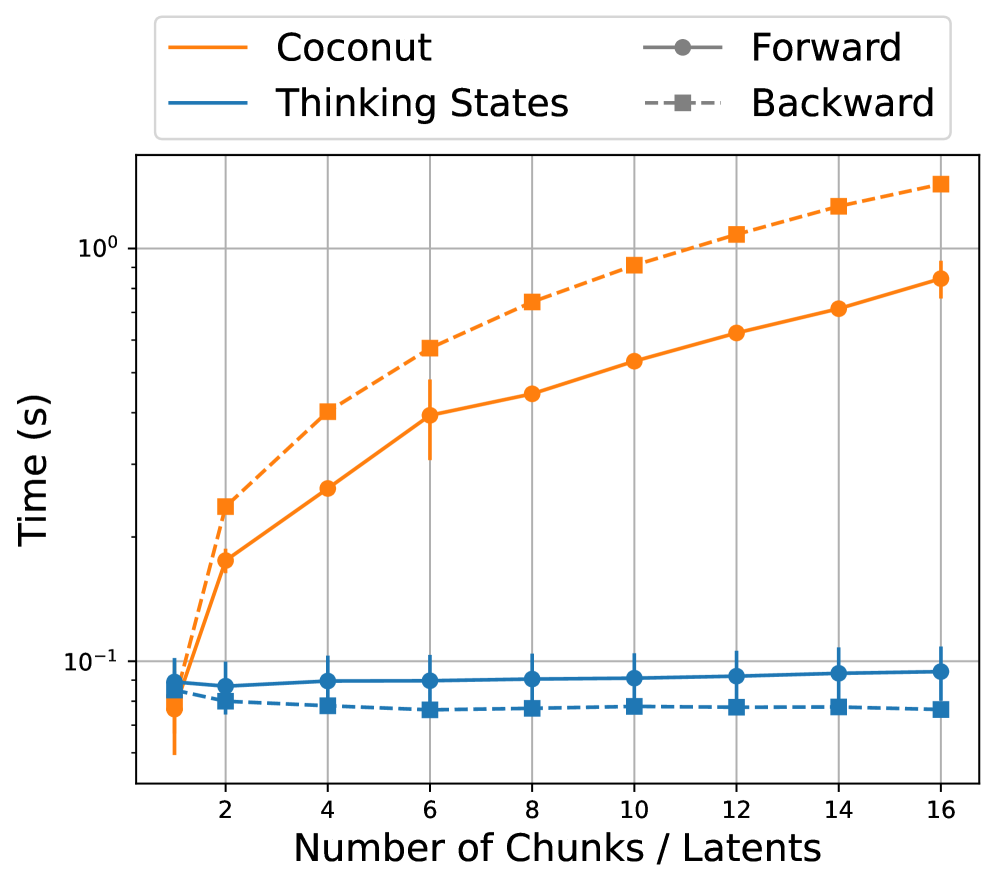
The image is a line chart comparing the computational time (in seconds) of two methods, "Coconut" and "Thinking States," as a function of problem size ("Number of Chunks / Latents"). Each method is further broken down into "Forward" and "Backward" passes. The chart uses a logarithmic scale for the time axis.
### Components/Axes
* **Chart Type:** Line chart with error bars.
* **X-Axis:**
* **Label:** `Number of Chunks / Latents`
* **Scale:** Linear, with major tick marks at 2, 4, 6, 8, 10, 12, 14, and 16.
* **Y-Axis:**
* **Label:** `Time (s)`
* **Scale:** Logarithmic (base 10), ranging from `10^-1` (0.1 seconds) to `10^0` (1.0 second).
* **Legend (Positioned at the top center of the chart area):**
* **Coconut:** Represented by an orange line.
* **Thinking States:** Represented by a blue line.
* **Forward:** Represented by a solid line with circular markers (●).
* **Backward:** Represented by a dashed line with square markers (■).
* **Combined Interpretation:** The legend defines four distinct data series:
1. **Coconut Forward:** Orange solid line with circle markers.
2. **Coconut Backward:** Orange dashed line with square markers.
3. **Thinking States Forward:** Blue solid line with circle markers.
4. **Thinking States Backward:** Blue dashed line with square markers.
### Detailed Analysis
**Data Series & Trends:**
1. **Coconut Forward (Orange, Solid, Circles):**
* **Trend:** Shows a strong, approximately linear upward trend on the logarithmic scale, indicating an exponential increase in time with the number of chunks/latents.
* **Approximate Data Points (with uncertainty from visual estimation):**
* At 1 chunk: ~0.08 s (with a large error bar extending below 0.05 s).
* At 2 chunks: ~0.15 s.
* At 4 chunks: ~0.25 s.
* At 6 chunks: ~0.35 s.
* At 8 chunks: ~0.45 s.
* At 10 chunks: ~0.55 s.
* At 12 chunks: ~0.65 s.
* At 14 chunks: ~0.75 s.
* At 16 chunks: ~0.85 s.
2. **Coconut Backward (Orange, Dashed, Squares):**
* **Trend:** Also shows a strong, approximately linear upward trend on the logarithmic scale, parallel to but consistently higher than the Coconut Forward series.
* **Approximate Data Points:**
* At 1 chunk: ~0.1 s.
* At 2 chunks: ~0.2 s.
* At 4 chunks: ~0.35 s.
* At 6 chunks: ~0.5 s.
* At 8 chunks: ~0.65 s.
* At 10 chunks: ~0.8 s.
* At 12 chunks: ~1.0 s.
* At 14 chunks: ~1.1 s.
* At 16 chunks: ~1.2 s.
3. **Thinking States Forward (Blue, Solid, Circles):**
* **Trend:** Appears nearly flat, showing a very slight, almost negligible increase in time as the number of chunks/latents increases.
* **Approximate Data Points:** Consistently clustered around ~0.09 s across all x-axis values (from 1 to 16 chunks). Error bars are present but relatively small.
4. **Thinking States Backward (Blue, Dashed, Squares):**
* **Trend:** Appears completely flat, showing no discernible increase in time with problem size.
* **Approximate Data Points:** Consistently clustered around ~0.07 s across all x-axis values. This series is consistently the lowest in time.
### Key Observations
1. **Divergent Scaling:** The most prominent feature is the stark difference in scaling behavior. The "Coconut" method's time cost grows exponentially with problem size (linear on log plot), while the "Thinking States" method's time cost is nearly constant.
2. **Forward vs. Backward Cost:** For the "Coconut" method, the Backward pass is consistently more time-consuming than the Forward pass. For "Thinking States," the difference between Forward and Backward passes is minimal, with the Backward pass being slightly faster.
3. **Performance Crossover:** At the smallest problem size (1 chunk), the times for all methods are relatively close (within the 0.05-0.1 s range). As the number of chunks increases, the performance gap widens dramatically, with "Coconut" becoming orders of magnitude slower than "Thinking States" at 16 chunks.
4. **Error Bars:** The "Coconut" series, particularly at lower chunk counts, show larger error bars, suggesting higher variance in its execution time compared to the more stable "Thinking States" method.
### Interpretation
This chart demonstrates a fundamental difference in the algorithmic complexity or implementation efficiency between the "Coconut" and "Thinking States" approaches for the measured task.
* **"Coconut"** exhibits **poor scalability**. Its computational time increases exponentially with the problem size (number of chunks/latents). This suggests its algorithm has a high time complexity (e.g., O(n^k) where k>1), making it increasingly impractical for larger problems. The higher cost of the Backward pass might indicate a more complex gradient computation or optimization step.
* **"Thinking States"** exhibits **excellent, near-constant-time scalability**. Its performance is largely independent of the problem size within the tested range. This is characteristic of algorithms with O(1) or very low O(log n) complexity for this parameter. This property is highly desirable, as it means the method can handle larger inputs without a significant performance penalty. The minimal difference between Forward and Backward passes suggests a symmetric and efficient computation.
**Conclusion:** The data strongly suggests that for tasks involving a variable number of "Chunks / Latents," the "Thinking States" method is vastly more efficient and scalable than the "Coconut" method. The choice between them would heavily depend on the expected problem size; for small, fixed-size problems, the difference may be negligible, but for any application where the input size can grow, "Thinking States" is the clearly superior choice from a performance perspective.