# Technical Data Extraction: MSE vs. Pilot Size Performance Chart
## 1. Image Overview
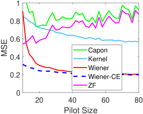
This image is a line graph illustrating the relationship between **Pilot Size** (independent variable) and **MSE** (Mean Squared Error, dependent variable) for five different signal processing or estimation algorithms.
## 2. Component Isolation
### A. Axis Labels and Markers
* **Y-Axis (Vertical):**
* **Label:** `MSE`
* **Scale:** Linear, ranging from `0` to `1`.
* **Major Tick Marks:** `0`, `0.2`, `0.4`, `0.6`, `0.8`, `1`.
* **X-Axis (Horizontal):**
* **Label:** `Pilot Size`
* **Scale:** Linear, ranging from approximately `10` to `80`.
* **Major Tick Marks:** `20`, `40`, `60`, `80`.
### B. Legend (Spatial Grounding: Center-Right [~650, 550])
The legend is contained within a black-bordered box and identifies five data series:
1. **Capon:** Solid Green line.
2. **Kernel:** Solid Light Blue line.
3. **Wiener:** Solid Red line.
4. **Wiener-CE:** Dashed Dark Blue line.
5. **ZF:** Solid Magenta line.
---
## 3. Data Series Analysis and Trends
### Capon (Solid Green Line)
* **Trend:** Highly volatile with a general downward slope initially, followed by significant fluctuations. It maintains the highest MSE throughout most of the range.
* **Key Points:** Starts near `1.0` at low pilot sizes, drops to ~`0.75` around pilot size 20, then fluctuates between `0.8` and `1.0` for the remainder of the plot.
### Kernel (Solid Light Blue Line)
* **Trend:** Smooth, monotonic decrease.
* **Key Points:** Starts at ~`0.85` (Pilot Size 10) and steadily declines to ~`0.58` (Pilot Size 80). It shows the most consistent improvement as pilot size increases without the noise seen in Capon or ZF.
### Wiener (Solid Red Line)
* **Trend:** Sharp exponential-like decay, flattening out at higher pilot sizes.
* **Key Points:** Starts very high (~`0.9` at Pilot Size 10), drops rapidly to ~`0.3` by Pilot Size 20, and eventually converges with the Wiener-CE line at ~`0.2` for Pilot Sizes > 60.
### Wiener-CE (Dashed Dark Blue Line)
* **Trend:** Gradual, smooth decrease. This is the best-performing algorithm across the entire range.
* **Key Points:** Starts at the lowest point (~`0.32` at Pilot Size 10) and slowly declines to a floor of ~`0.2` at Pilot Size 80.
### ZF (Solid Magenta Line)
* **Trend:** Highly volatile with an overall upward (worsening) trend as pilot size increases.
* **Key Points:** Starts at ~`0.55` (Pilot Size 10). Despite some dips, it trends upward, ending near ~`0.9` at Pilot Size 80. This suggests the Zero Forcing (ZF) method performs worse or becomes more unstable as the pilot size grows in this specific context.
---
## 4. Comparative Summary Table
| Algorithm | Color/Style | Initial MSE (approx.) | Final MSE (approx.) | Stability |
| :--- | :--- | :--- | :--- | :--- |
| **Wiener-CE** | Dashed Blue | 0.32 | 0.20 | Very Stable (Best) |
| **Wiener** | Solid Red | 0.90 | 0.20 | High initial error, converges to best |
| **Kernel** | Solid Light Blue | 0.85 | 0.58 | Stable/Predictable |
| **Capon** | Solid Green | 1.00 | 0.95 | Highly Volatile (Worst) |
| **ZF** | Solid Magenta | 0.55 | 0.90 | Volatile/Degrading |
## 5. Technical Observations
* **Convergence:** The `Wiener` and `Wiener-CE` algorithms converge to the same minimum error floor of approximately `0.2` as the Pilot Size exceeds 60.
* **Performance Gap:** There is a significant performance gap (approx. 0.4 MSE units) between the Wiener-based methods and the other three methods (Capon, Kernel, ZF) at larger pilot sizes.
* **Anomalous Trend:** The `ZF` (Magenta) line is unique in that its performance generally degrades (MSE increases) as the Pilot Size increases, whereas most estimation models typically improve with more data.