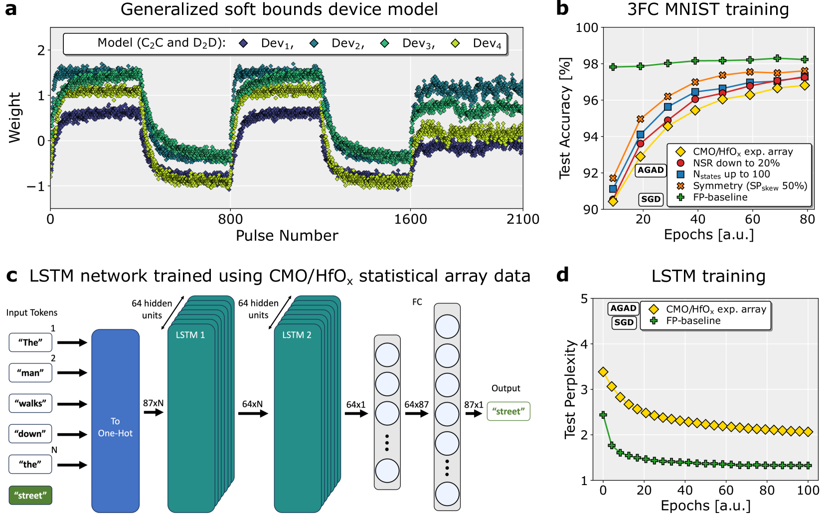
## [Multi-Panel Technical Figure]: Device Modeling and Neural Network Training Performance ### Overview This image is a composite figure containing four panels (a, b, c, d) that collectively present data on a generalized device model, its application in training neural networks (3FC on MNIST and an LSTM), and the resulting performance metrics. The figure combines line charts and a network architecture diagram. ### Components/Axes The figure is divided into four quadrants: * **Panel a (Top-Left):** A line chart titled "Generalized soft bounds device model". * **Panel b (Top-Right):** A line chart titled "3FC MNIST training". * **Panel c (Bottom-Left):** A schematic diagram titled "LSTM network trained using CMO/HfOₓ statistical array data". * **Panel d (Bottom-Right):** A line chart titled "LSTM training". ### Detailed Analysis #### **Panel a: Generalized soft bounds device model** * **Chart Type:** Line chart with multiple data series. * **Y-Axis:** Label: "Weight". Scale ranges from -1 to 2, with major ticks at -1, 0, 1, 2. * **X-Axis:** Label: "Pulse Number". Scale ranges from 0 to 2100, with major ticks at 0, 800, 1600, 2100. * **Legend:** Located in the top-left corner. Title: "Model (C₂C and D₂D):". It defines four data series: * `Dev₁`: Dark blue diamond (♦) * `Dev₂`: Teal diamond (♦) * `Dev₃`: Green diamond (♦) * `Dev₄`: Yellow-green diamond (♦) * **Data Trends & Points:** All four series show a similar pattern of oscillation. They start near a weight of 0, rise to a plateau between ~0.5 and 1.5, drop sharply to a trough between ~-1 and 0, rise again to a second plateau, drop to a second trough, and finally rise to a third plateau. The series are vertically offset from each other, with `Dev₄` (yellow-green) generally having the highest weight values and `Dev₁` (dark blue) the lowest during the plateau phases. The data points are densely plotted, creating thick, noisy bands rather than single lines. #### **Panel b: 3FC MNIST training** * **Chart Type:** Line chart with multiple data series. * **Y-Axis:** Label: "Test Accuracy [%]". Scale ranges from 90 to 100, with major ticks every 2 units. * **X-Axis:** Label: "Epochs [a.u.]". Scale ranges from 0 to 80, with major ticks at 0, 20, 40, 60, 80. * **Legend:** Located in the bottom-right corner. It defines five data series and includes two annotations ("AGAD", "SGD") pointing to specific lines. * `CMO/HfOₓ exp. array`: Yellow diamond (♦) * `NSR down to 20%`: Red circle (●) * `Nstates up to 100`: Blue square (■) * `Symmetry (SPskew 50%)`: Orange cross (✖) * `FP-baseline`: Green plus (+) * **Data Trends & Points:** * **Trend:** All lines show increasing test accuracy with more epochs, with the rate of increase slowing over time (diminishing returns). They appear to converge towards the end of training (80 epochs). * **Key Points (Approximate at 80 Epochs):** * `FP-baseline` (Green +): Highest accuracy, ~98.5%. * `Symmetry (SPskew 50%)` (Orange ✖): ~97.8%. * `Nstates up to 100` (Blue ■): ~97.5%. * `NSR down to 20%` (Red ●): ~97.2%. * `CMO/HfOₓ exp. array` (Yellow ♦): Lowest accuracy, ~96.8%. * **Annotations:** The label "AGAD" points to the yellow diamond line (`CMO/HfOₓ exp. array`). The label "SGD" points to the green plus line (`FP-baseline`). #### **Panel c: LSTM network trained using CMO/HfOₓ statistical array data** * **Diagram Type:** Neural network architecture schematic. * **Components & Flow (Left to Right):** 1. **Input Tokens:** A vertical list of text boxes: `"The"`, `"man"`, `"walks"`, `"down"`, `"the"`. A green box at the bottom contains the target word `"street"`. 2. **To One-Hot:** A blue rectangular block. Arrows from each input token point to this block. An arrow labeled `87xN` points from this block to the next layer. 3. **LSTM 1:** A stack of teal rectangles labeled "LSTM 1". An annotation points to it: "64 hidden units". An arrow labeled `64xN` points to the next layer. 4. **LSTM 2:** A stack of teal rectangles labeled "LSTM 2". An annotation points to it: "64 hidden units". An arrow labeled `64x1` points to the next layer. 5. **FC (Fully Connected) Layer:** A vertical column of circles (neurons). An arrow labeled `64x87` points from this to the next layer. 6. **Output Layer:** A vertical column of circles. An arrow labeled `87x1` points from this to the final output. 7. **Output:** A green text box containing the predicted word `"street"`. * **Text Transcription:** All text within the diagram is in English. The input sequence is: "The", "man", "walks", "down", "the". The target/output is: "street". #### **Panel d: LSTM training** * **Chart Type:** Line chart with two data series. * **Y-Axis:** Label: "Test Perplexity". Scale ranges from 1 to 5, with major ticks at 1, 2, 3, 4, 5. * **X-Axis:** Label: "Epochs [a.u.]". Scale ranges from 0 to 100, with major ticks at 0, 20, 40, 60, 80, 100. * **Legend:** Located in the top-left corner. It defines two data series and includes annotations ("AGAD", "SGD"). * `CMO/HfOₓ exp. array`: Yellow diamond (♦) * `FP-baseline`: Green plus (+) * **Data Trends & Points:** * **Trend:** Both lines show decreasing test perplexity (lower is better) with more epochs, with the rate of decrease slowing over time. * **Key Points (Approximate):** * `FP-baseline` (Green +): Starts at ~2.4, drops rapidly, and plateaus near ~1.3 by epoch 100. * `CMO/HfOₓ exp. array` (Yellow ♦): Starts higher at ~3.4, drops steadily, and plateaus near ~2.0 by epoch 100. It remains consistently above the baseline throughout training. * **Annotations:** The label "AGAD" points to the yellow diamond line (`CMO/HfOₓ exp. array`). The label "SGD" points to the green plus line (`FP-baseline`). ### Key Observations 1. **Performance Hierarchy:** In both training tasks (3FC MNIST and LSTM), the `FP-baseline` (ideal software model) outperforms the hardware-inspired `CMO/HfOₓ exp. array` model. The experimental array shows lower accuracy and higher perplexity. 2. **Impact of Non-Idealities:** Panel b suggests that modifying specific non-idealities (like Noise-to-Signal Ratio - NSR, number of states - Nstates, or symmetry) in the model brings performance closer to the baseline, but not fully to it. 3. **Device Behavior:** Panel a shows that the generalized device model (`Dev₁` to `Dev₄`) exhibits bounded, oscillatory weight updates in response to pulses, which is characteristic of memristive or analog memory devices. The vertical offset between devices suggests device-to-device variability. 4. **Convergence:** All training curves (Panels b and d) show clear convergence, indicating the models have learned stably from the data. ### Interpretation This figure demonstrates the process and challenges of mapping ideal neural network algorithms onto non-ideal, hardware-inspired device models. Panel **a** establishes the fundamental, noisy, and bounded behavior of the underlying device. Panels **b** and **d** then show the direct consequence of using such devices (or statistical models thereof) for training: a measurable degradation in final model performance (accuracy/perplexity) compared to a perfect software baseline (`FP-baseline`). The intermediate lines in Panel **b** are crucial—they act as an ablation study, isolating which specific hardware non-idealities (noise, limited states, asymmetry) contribute most to the performance gap. The LSTM diagram in Panel **c** provides the architectural context for the results in Panel **d**. The overall narrative is one of **characterization and mitigation**: understanding device-level constraints (a) and quantifying their system-level impact (b, d) to guide the design of more robust algorithms or better devices. The persistent gap between the experimental array and the baseline highlights the ongoing challenge in achieving software-equivalent performance with analog hardware.