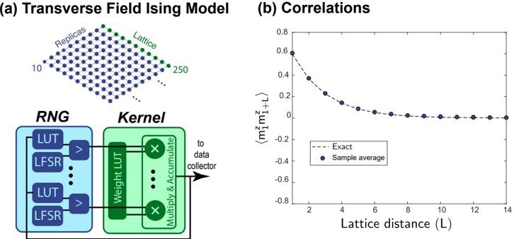
\n ## Diagram & Chart: Transverse Field Ising Model & Correlations ### Overview The image presents two related components: (a) a diagram illustrating the structure of a Transverse Field Ising Model simulation, including a Random Number Generator (RNG) and Kernel, and (b) a chart displaying correlations as a function of lattice distance. The diagram shows the flow of data from the RNG to the Kernel, while the chart presents a comparison between exact calculations and sample averages of correlation values. ### Components/Axes **(a) Diagram:** * **RNG (Random Number Generator):** Composed of two LFSR (Linear Feedback Shift Register) blocks and two LUT (Lookup Table) blocks. * **Kernel:** Contains a "Weight LUT" and "Multiply & Accumulate" blocks. * **Replicas:** A diagonal axis labeled "Replicas" ranging from approximately 10 to 250. * **Lattice:** A diagonal axis labeled "Lattice" ranging from approximately 10 to 250. * **Arrows:** Indicate the flow of data from the RNG to the Kernel and then "to collector". **(b) Chart:** * **X-axis:** "Lattice distance (L)", ranging from 2 to 14. * **Y-axis:** "(mᵢmᵢ₊₁₋L)", ranging from -0.8 to 0.8. * **Legend:** * "Exact" - Represented by a dashed black line. * "Sample average" - Represented by blue circles. ### Detailed Analysis or Content Details **(a) Diagram:** The RNG section consists of two LFSR blocks connected to two LUT blocks via ">" symbols, likely representing a comparison or transformation. The output of the LUTs feeds into the Kernel. The Kernel contains a "Weight LUT" and a "Multiply & Accumulate" block, suggesting a weighted summation process. The output of the Kernel is directed "to collector". The diagonal axes labeled "Replicas" and "Lattice" suggest a simulation setup involving multiple replicas and a lattice structure. The axes are not linear, and the values are approximate. **(b) Chart:** The dashed black line ("Exact") starts at approximately 0.68 at L=2 and decreases rapidly, crossing the x-axis around L=4. It continues to decrease, approaching approximately -0.1 at L=14. The blue circles ("Sample average") follow a similar trend, starting at approximately 0.65 at L=2. The sample average line is more noisy than the exact line, but generally tracks the exact line. At L=2, the sample average is approximately 0.65. At L=4, the sample average is approximately 0.2. At L=6, the sample average is approximately -0.1. At L=8, the sample average is approximately -0.2. At L=10, the sample average is approximately -0.25. At L=12, the sample average is approximately -0.25. At L=14, the sample average is approximately -0.1. ### Key Observations * The "Exact" and "Sample average" lines show a strong correlation, but the sample average exhibits more fluctuation. * The correlation values decrease with increasing lattice distance, eventually becoming negative. * The diagram suggests a computational setup for simulating the Transverse Field Ising Model, with a focus on generating random numbers and applying a kernel function. * The diagonal axes in the diagram suggest a relationship between the number of replicas and the lattice size. ### Interpretation The image illustrates a computational approach to studying the Transverse Field Ising Model. The diagram outlines the key components of the simulation, including a random number generator and a kernel function. The chart presents the results of the simulation, specifically the correlation between spins at different lattice distances. The decreasing correlation with increasing distance suggests that the system exhibits short-range order. The comparison between the "Exact" and "Sample average" lines indicates the accuracy of the simulation. The fluctuations in the "Sample average" line are likely due to statistical noise, which can be reduced by increasing the number of samples. The model is likely used to study phase transitions and critical phenomena in magnetic materials. The use of replicas suggests a technique to average over different configurations or disorder. The overall setup suggests a Monte Carlo simulation approach to solving the Ising model.