TECHNICAL ASSET FINGERPRINT
4a5eb3c472df10f45fa05a9b
Click to view fullscreen
Press ESC or click to close
FOUND IN PAPERS
EXPERT: healer-alpha-free VERSION 1
RUNTIME: free/openrouter/healer-alpha
INTEL_VERIFIED
## [Multi-Panel Technical Figure]: CMO-HfOx ReRAM Programming Analysis
### Overview
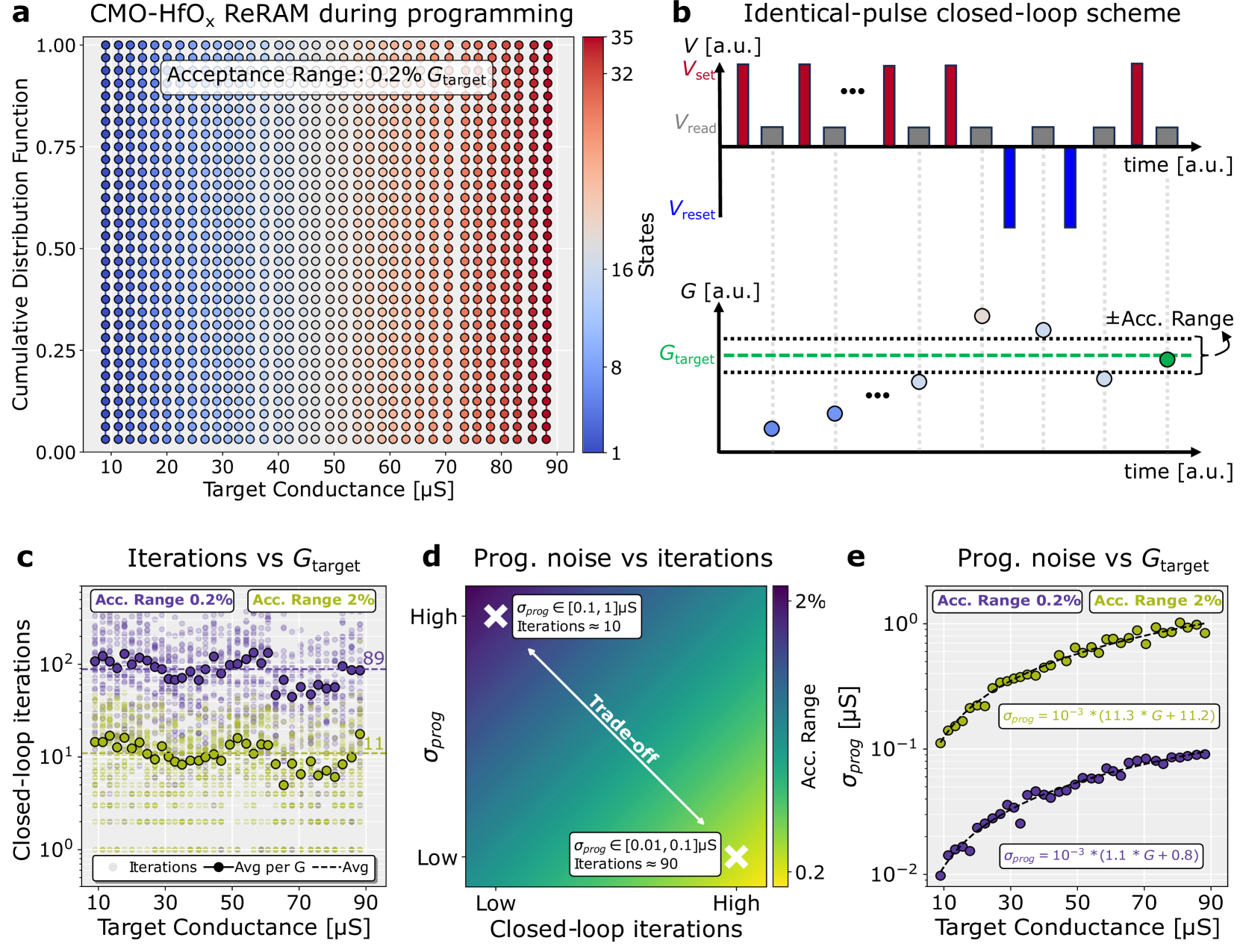
This composite figure presents a technical analysis of programming a CMO-HfOx Resistive Random-Access Memory (ReRAM) device using a closed-loop, identical-pulse scheme. It includes a conductance state distribution map, a schematic of the programming protocol, and three plots analyzing the relationship between programming iterations, target conductance, and programming noise (σ_prog) under different acceptance ranges.
### Components/Axes
The figure is divided into five panels labeled **a** through **e**.
**Panel a: CMO-HfOx ReRAM during programming**
* **Type:** 2D Heatmap / Scatter Plot.
* **X-axis:** "Target Conductance [µS]". Linear scale from 10 to 90 µS, with major ticks every 10 µS.
* **Y-axis:** "Cumulative Distribution Function". Linear scale from 0.00 to 1.00, with major ticks every 0.25.
* **Color Bar (Right):** Labeled "States". A vertical gradient from blue (bottom, value 1) to red (top, value 35). Major ticks at 1, 8, 16, 32, 35.
* **Legend/Annotation:** A text box in the upper portion reads: "Acceptance Range: 0.2% G_target".
* **Data Representation:** A grid of colored dots. Each column corresponds to a specific target conductance (G_target). The color of the dots in a column indicates the number of discrete conductance states (from 1 to 35) achieved for that target. The vertical spread (CDF) shows the distribution of programmed states.
**Panel b: Identical-pulse closed-loop scheme**
* **Type:** Two aligned schematic diagrams.
* **Top Graph (Voltage vs. Time):**
* **Y-axis:** "V [a.u.]" (arbitrary units). Labels: "V_set" (positive red pulses), "V_read" (smaller grey pulses), "V_reset" (negative blue pulses).
* **X-axis:** "time [a.u.]".
* **Flow:** Shows a sequence: a V_set pulse, followed by a V_read pulse, repeated multiple times (indicated by "..."), then a V_reset pulse, followed by a V_read pulse, and so on.
* **Bottom Graph (Conductance vs. Time):**
* **Y-axis:** "G [a.u.]". A horizontal green dashed line is labeled "G_target". Two horizontal black dotted lines above and below it define the "±Acc. Range".
* **X-axis:** "time [a.u.]". Aligned with the top graph.
* **Data Representation:** Circles represent measured conductance after each pulse. The circles change color from blue to green as they approach G_target. The final circle is solid green, within the acceptance range.
**Panel c: Iterations vs G_target**
* **Type:** Scatter Plot with overlaid trend lines.
* **X-axis:** "Target Conductance [µS]". Linear scale from 10 to 90 µS.
* **Y-axis:** "Closed-loop iterations". Logarithmic scale from 10^0 (1) to 10^2 (100).
* **Legend (Top):** Two colored boxes: "Acc. Range 0.2%" (purple) and "Acc. Range 2%" (yellow-green).
* **Legend (Bottom):** "Iterations" (small dots), "Avg per G" (solid line with circle markers), "---Avg" (dashed line).
* **Data Series:**
1. **Purple dots/line (0.2% range):** Data points are scattered between ~10 and ~100 iterations. The average line ("Avg per G") fluctuates around 80-90 iterations. A horizontal dashed line labeled "89" indicates the overall average.
2. **Yellow-green dots/line (2% range):** Data points are scattered between ~1 and ~20 iterations. The average line fluctuates around 10-15 iterations. A horizontal dashed line labeled "11" indicates the overall average.
**Panel d: Prog. noise vs iterations**
* **Type:** 2D Heatmap / Contour Plot.
* **X-axis:** "Closed-loop iterations". Labeled "Low" to "High".
* **Y-axis:** "σ_prog" (Programming noise). Labeled "Low" to "High".
* **Color Bar (Right):** Labeled "Acc. Range". Scale from 0.2 (blue) to 2% (yellow).
* **Annotations:**
* A white double-headed arrow labeled "Trade-off" runs diagonally from the bottom-left (low iterations, low noise) to the top-right (high iterations, high noise).
* **Top-left (High noise, Low iterations):** A white 'X' and text box: "σ_prog ∈ [0.1, 1]µS, Iterations ≈ 10".
* **Bottom-right (Low noise, High iterations):** A white 'X' and text box: "σ_prog ∈ [0.01, 0.1]µS, Iterations ≈ 90".
**Panel e: Prog. noise vs G_target**
* **Type:** Scatter Plot with fitted power-law curves.
* **X-axis:** "Target Conductance [µS]". Linear scale from 10 to 90 µS.
* **Y-axis:** "σ_prog [µS]". Logarithmic scale from 10^-2 (0.01) to 10^0 (1).
* **Legend (Top):** Same as Panel c: "Acc. Range 0.2%" (purple) and "Acc. Range 2%" (yellow-green).
* **Data Series & Equations:**
1. **Purple dots (0.2% range):** Data points follow an upward trend. A fitted curve is annotated with the equation: `σ_prog = 10^-3 * (1.1 * G + 0.8)`.
2. **Yellow-green dots (2% range):** Data points follow a steeper upward trend. A fitted curve is annotated with the equation: `σ_prog = 10^-3 * (11.3 * G + 11.2)`.
### Detailed Analysis
* **Panel a:** Shows that for a given target conductance (G_target), the programming process can settle into one of many discrete states (1-35). The color gradient indicates that higher target conductances (right side, ~70-90 µS) are associated with a higher number of possible states (red, ~32-35), while lower targets (left side, ~10-30 µS) are associated with fewer states (blue, ~1-16). The CDF shows the probability distribution across these states for each G_target.
* **Panel b:** Illustrates the feedback control loop. A set pulse (V_set) is applied, the conductance is read (V_read), and this is repeated until the measured conductance (G) falls within the predefined acceptance range (±Acc. Range) around the target (G_target). Reset pulses (V_reset) are interspersed, likely to prevent saturation or for device conditioning.
* **Panel c:** Demonstrates a clear trade-off. Achieving a tighter acceptance range (0.2%) requires significantly more programming iterations (average ~89) compared to a looser range (2%, average ~11). The number of iterations is relatively constant across the range of target conductances (10-90 µS) for a given acceptance range, though with considerable scatter.
* **Panel d:** Conceptualizes the fundamental trade-off between programming precision (low σ_prog) and speed (low iterations). High precision (low noise) demands many iterations, while fast programming (few iterations) results in higher noise. The color indicates that the 0.2% acceptance range (blue) corresponds to the high-iteration, low-noise regime, while the 2% range (yellow) corresponds to the low-iteration, high-noise regime.
* **Panel e:** Quantifies the relationship between programming noise and target conductance. For both acceptance ranges, σ_prog increases linearly with G_target (on a log-linear plot, indicating a power-law relationship). The slope is much steeper for the 2% acceptance range (coefficient 11.3) than for the 0.2% range (coefficient 1.1), meaning noise worsens more rapidly with increasing conductance when the precision requirement is relaxed.
### Key Observations
1. **Discrete States:** The ReRAM device programs into a finite number of discrete conductance states, not a continuous range.
2. **Precision-Speed Trade-off:** There is an inverse relationship between programming precision (acceptance range/noise) and programming speed (iterations). This is explicitly highlighted in Panel d.
3. **Noise Scaling:** Programming noise (σ_prog) scales linearly with the target conductance value. The scaling factor is heavily dependent on the required precision (acceptance range).
4. **Iteration Consistency:** The number of iterations required to reach a target is largely independent of the target conductance value itself for a fixed acceptance range (Panel c), but the resulting noise is not (Panel e).
### Interpretation
This figure characterizes the performance and fundamental limits of a specific closed-loop programming algorithm for CMO-HfOx ReRAM. The data suggests that:
* **For applications requiring high precision (e.g., analog computing weights):** One must use a tight acceptance range (0.2%), which will result in slower programming (~89 iterations) but lower absolute noise levels, especially at lower conductance values.
* **For applications prioritizing speed (e.g., digital memory):** A looser acceptance range (2%) can be used, enabling much faster programming (~11 iterations), but at the cost of higher conductance variability (noise), which scales poorly with increasing conductance.
* **Device Physics Insight:** The linear scaling of σ_prog with G_target (Panel e) may reflect underlying physical mechanisms in the ReRAM filament formation/modulation, where achieving higher conductance states inherently involves more variability. The fitted equations provide a predictive model for noise based on target conductance and desired precision.
* **System Design Implication:** The clear trade-off (Panel d) presents a design knob for system architects. They can choose an operating point on the precision-speed curve based on the specific requirements of the neural network or computing task being implemented on the ReRAM array. The data in Panels c and e provide the quantitative basis for making that choice.
DECODING INTELLIGENCE...