## Line Chart: Throughput vs. Block Size (b) for varying Matrix Sizes (m)
### Overview
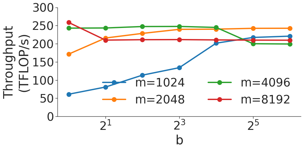
This image is a line chart illustrating the relationship between computational throughput (measured in TFLOP/s) and a variable 'b' (likely block size or a parallelization parameter) across four different matrix sizes 'm' (1024, 2048, 4096, 8192). The chart demonstrates how throughput scales as 'b' increases, with different behaviors observed depending on the value of 'm'.
### Components/Axes
* **Y-Axis:** Labeled "Throughput (TFLOP/s)". The scale ranges from 0 to 300, with major grid lines at intervals of 50.
* **X-Axis:** Labeled "b". The scale is logarithmic, with explicit markers at $2^1$, $2^3$, and $2^5$.
* **Legend:** Located in the center-right area of the chart.
* **Blue line:** $m=1024$
* **Orange line:** $m=2048$
* **Green line:** $m=4096$
* **Red line:** $m=8192$
### Detailed Analysis
The chart contains four data series, each consisting of 7 data points.
**1. Blue Line ($m=1024$)**
* **Trend:** This line shows a consistent, steady upward trend across the entire X-axis range.
* **Data Points (Approximate):**
* Starts at $b \approx 2^0$ with a throughput of $\approx 60$ TFLOP/s.
* Increases steadily through $b \approx 2^1$ ($\approx 80$), $b \approx 2^2$ ($\approx 115$), and $b \approx 2^3$ ($\approx 135$).
* Shows a sharper increase between $b \approx 2^3$ and $b \approx 2^4$, reaching $\approx 200$ TFLOP/s.
* Flattens out at the end near $\approx 220$ TFLOP/s.
**2. Orange Line ($m=2048$)**
* **Trend:** Starts with a sharp upward slope, then transitions to a gradual, shallow upward trend, eventually saturating.
* **Data Points (Approximate):**
* Starts at $b \approx 2^0$ with a throughput of $\approx 170$ TFLOP/s.
* Jumps to $\approx 215$ TFLOP/s at $b \approx 2^1$.
* Continues a slow, steady climb from $\approx 225$ TFLOP/s to $\approx 240$ TFLOP/s as 'b' increases toward $2^5$.
**3. Green Line ($m=4096$)**
* **Trend:** Starts high and remains stable (flat) for the first half of the X-axis, then experiences a sharp drop-off.
* **Data Points (Approximate):**
* Starts at $b \approx 2^0$ with a throughput of $\approx 245$ TFLOP/s.
* Remains stable at $\approx 245$ TFLOP/s until $b \approx 2^4$.
* Drops sharply at the final data point ($b \approx 2^5$) to $\approx 200$ TFLOP/s.
**4. Red Line ($m=8192$)**
* **Trend:** Starts at the highest throughput value, drops sharply immediately, and then remains stable (flat).
* **Data Points (Approximate):**
* Starts at $b \approx 2^0$ with a throughput of $\approx 260$ TFLOP/s.
* Drops sharply to $\approx 210$ TFLOP/s at $b \approx 2^1$.
* Remains stable at $\approx 210$ TFLOP/s for the remainder of the X-axis range.
### Key Observations
* **Crossover Points:** There is a significant convergence of performance around the $b \approx 2^4$ to $2^5$ range, where all four lines cluster between 200 and 240 TFLOP/s.
* **Performance Inversion:** At low 'b' values, larger 'm' values (8192, 4096) provide significantly higher throughput than smaller 'm' values (1024). However, as 'b' increases, the smaller 'm' values catch up, and the larger 'm' values actually see a performance degradation (the "cliff" in the Red and Green lines).
* **Saturation:** The Orange ($m=2048$) and Blue ($m=1024$) lines appear to be approaching a saturation point, suggesting that increasing 'b' further may yield diminishing returns.
### Interpretation
This data likely represents a performance benchmark for a parallel computing operation, such as matrix multiplication on a GPU or similar accelerator.
* **The "m" variable:** Likely represents the matrix size. Larger matrices (8192) are more efficient at low block sizes ('b') because they can better saturate the hardware's compute units.
* **The "b" variable:** Likely represents a block size or tiling factor.
* **The "Cliff" (Red/Green lines):** The sharp drop in throughput for larger matrices as 'b' increases suggests that the block size has become too large, likely causing cache thrashing, memory bandwidth bottlenecks, or overhead in the parallelization logic.
* **The "Growth" (Blue line):** The smaller matrix ($m=1024$) requires a larger block size ('b') to achieve optimal hardware utilization, which is why it shows a positive slope while the others are flat or declining.
In summary, there is an "optimal" 'b' for each 'm'. For smaller matrices, you need a larger 'b' to reach peak performance; for larger matrices, a smaller 'b' is preferred to avoid performance penalties.