## Diagram: Computational Imaging System Architecture
### Overview
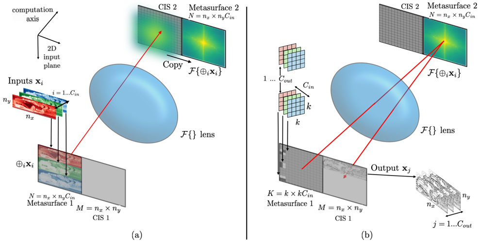
The image depicts two diagrams (a) and (b) illustrating a computational imaging system. Both diagrams show inputs passing through a lens (`F{}`) and interacting with metasurfaces and computational imaging sensors (CIS) to produce outputs. Diagram (a) focuses on input-output relationships, while diagram (b) introduces additional processing layers (e.g., a grid labeled `k` and `C_out`).
### Components/Axes
#### Diagram (a):
- **Inputs**: Labeled `x_i` (2D input plane) with dimensions `n_x × n_y × C_in`.
- **Lens**: Central blue oval labeled `F{}` (function mapping).
- **Metasurfaces**:
- Metasurface 1: Dimensions `M = n_x × n_y`, labeled `CIS 1`.
- Metasurface 2: Dimensions `N = n_x × n_y × C_in`, labeled `CIS 2`.
- **Outputs**: Labeled `x_j` with dimensions `n_x × n_y`.
- **Arrows**: Red arrows indicate flow from inputs → lens → metasurfaces → outputs.
#### Diagram (b):
- **Inputs**: Same as (a), but with an additional grid labeled `k` (size `K = k × C_in`).
- **Processing Layer**: Grid labeled `C_out` (output channels).
- **Outputs**: Structured as `n_x × n_y` with hierarchical layers (e.g., `j = 1...C_out`).
- **Arrows**: Red arrows show flow from inputs → grid → lens → metasurfaces → outputs.
### Detailed Analysis
#### Diagram (a):
- **Inputs**: 2D input plane (`x_i`) with spatial dimensions `n_x × n_y` and `C_in` channels.
- **Metasurface 1**: Acts as a first-stage processor (`CIS 1`), preserving spatial dimensions (`M = n_x × n_y`).
- **Metasurface 2**: Adds channel depth (`N = n_x × n_y × C_in`), suggesting feature extraction or modulation.
- **Lens (`F{}`)**: Central processing unit, likely applying a transformation (e.g., Fourier or phase modulation).
#### Diagram (b):
- **Grid (`k`)**: Introduces a parameterized layer (`K = k × C_in`), possibly for adaptive filtering or parameter tuning.
- **Output Structure**: Hierarchical output (`j = 1...C_out`) implies multi-scale or multi-feature outputs.
- **Lens (`F{}`)**: Retains central role but interacts with the grid before metasurface processing.
### Key Observations
1. **Flow Consistency**: Both diagrams show inputs passing through the lens before metasurface processing, but (b) adds a grid-based preprocessing step.
2. **Dimensionality**:
- Metasurface 1: Maintains spatial resolution (`n_x × n_y`).
- Metasurface 2: Expands channel depth (`C_in`).
3. **Output Complexity**: Diagram (b) introduces a multi-channel output (`C_out`), suggesting advanced processing capabilities.
### Interpretation
The diagrams represent a computational imaging system where:
- **Inputs** (2D spatial data) are modulated by a lens (`F{}`) to encode spatial or spectral information.
- **Metasurfaces** manipulate light properties (e.g., phase, amplitude) to extract features.
- **Diagram (b)** enhances the system with a grid-based preprocessing layer (`k`), enabling adaptive control over the imaging process.
- The hierarchical output structure (`C_out`) in (b) suggests applications in multi-modal imaging (e.g., simultaneous capture of intensity and phase).
The system likely leverages metasurface-based computational imaging for tasks like hyperspectral imaging, 3D reconstruction, or adaptive optics. The inclusion of `k` in (b) implies tunable parameters for optimizing image quality or resolution.