\n
## Diagram: Neural Network Sparsity Illustration
### Overview
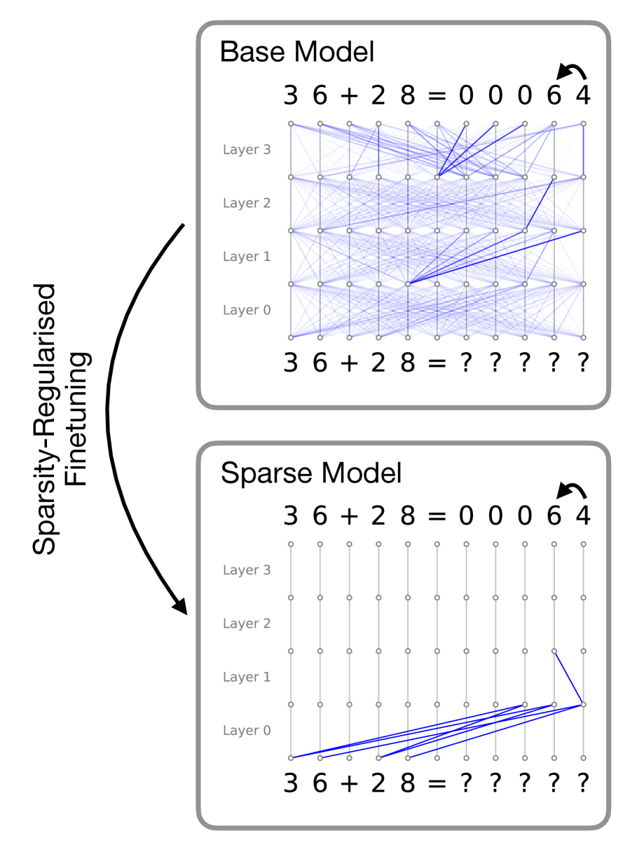
The image presents a diagram illustrating the effect of sparsity-regularized finetuning on a neural network. It compares a "Base Model" with a "Sparse Model," visually demonstrating how finetuning can reduce the number of active connections within the network. The diagram uses a layered network representation with connections between layers.
### Components/Axes
The diagram consists of two main sections: "Base Model" (top) and "Sparse Model" (bottom). Each section depicts a neural network with four layers labeled "Layer 0", "Layer 1", "Layer 2", and "Layer 3". Both sections show the input "3 6 + 2 8" and the output "0 0 0 6 4" with question marks in between. A curved arrow labeled "Sparsity-Regularised Finetuning" connects the two sections, indicating the transformation process. The connections between layers are represented by lines.
### Detailed Analysis or Content Details
**Base Model:**
* The base model shows a dense network with numerous connections between each layer. The lines representing connections are predominantly blue.
* Input: "3 6 + 2 8"
* Output: "0 0 0 6 4"
* Layer 0 has 8 nodes.
* Layer 1 has 8 nodes.
* Layer 2 has 8 nodes.
* Layer 3 has 8 nodes.
* Connections: Almost every node in one layer is connected to almost every node in the next layer.
**Sparse Model:**
* The sparse model shows a network with significantly fewer connections. The lines representing connections are predominantly blue, but much sparser than in the base model. A blue line is also present to indicate the trend of the connections.
* Input: "3 6 + 2 8"
* Output: "0 0 0 6 4"
* Layer 0 has 8 nodes.
* Layer 1 has 8 nodes.
* Layer 2 has 8 nodes.
* Layer 3 has 8 nodes.
* Connections: Only a subset of nodes in each layer are connected to nodes in the next layer. The connections are concentrated along a diagonal.
**Arrow:**
* The arrow labeled "Sparsity-Regularised Finetuning" is positioned on the left side of the diagram and curves from the "Base Model" to the "Sparse Model," indicating the direction of the transformation.
### Key Observations
* The primary difference between the two models is the density of connections. The base model is densely connected, while the sparse model has significantly fewer connections.
* The sparse model appears to have connections concentrated along a diagonal, suggesting that the finetuning process prioritizes certain pathways within the network.
* The input and output remain the same in both models, indicating that the finetuning process aims to achieve the same functionality with a more efficient network structure.
### Interpretation
The diagram illustrates the concept of model sparsity, a technique used to reduce the computational cost and memory footprint of neural networks. Sparsity-regularized finetuning encourages the network to learn a solution that relies on a smaller subset of connections, effectively pruning away redundant or less important pathways. This can lead to faster inference times and reduced energy consumption without sacrificing accuracy. The diagram visually demonstrates how this process transforms a dense network into a sparse one, highlighting the reduction in connections while maintaining the same input-output behavior. The concentration of connections along a diagonal in the sparse model suggests that the finetuning process has identified a set of key pathways that are sufficient for performing the task. The question marks in the middle of the input and output suggest that the internal workings of the network are being simplified, but the overall function remains the same.