## Diagram: Open-loop and Closed-loop CIM with Potential and Error Space Visualizations
### Overview
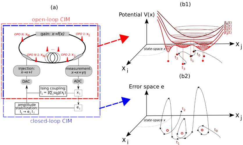
The image presents a schematic diagram of both open-loop and closed-loop Coherent Ising Machines (CIMs), accompanied by visualizations of the potential landscape and error space associated with the system's dynamics. The diagram is divided into three main sections: (a) showing the CIM configurations, (b1) illustrating the potential V(x), and (b2) illustrating the error space e.
### Components/Axes
#### Section (a): CIM Configurations
* **Title:** (a)
* **Sub-title:** open-loop CIM (enclosed in a dashed red box)
* **Sub-title:** closed-loop CIM (enclosed in a dashed blue box)
* **Components within the Open-loop CIM:**
* A circular loop representing the optical path.
* OPO N: XN (Optical Parametric Oscillator N, with output XN)
* gain: x→f(x) (Gain element, transforming input x to f(x))
* OPO 1: X1 (Optical Parametric Oscillator 1, with output X1)
* OPO N-1: XN/1 (Optical Parametric Oscillator N-1, with output XN/1)
* OPO 2: X2 (Optical Parametric Oscillator 2, with output X2)
* injection: x→x+l (Injection element, adding l to input x)
* measurement: x→x+γη (Measurement element, transforming input x to x+γη)
* DAC (Digital-to-Analog Converter)
* ADC (Analog-to-Digital Converter)
* Ising coupling: Ii = βΣjωijg(xj) (Ising coupling element, calculating Ii based on coupling strength β, weights ωij, and function g(xj))
* **Components within the Closed-loop CIM:**
* amplitude stabilization: Ii→eiIi (Amplitude stabilization element, transforming Ii to eiIi)
* ei (Error signal)
#### Section (b1): Potential V(x)
* **Title:** (b1)
* **Graph Title:** Potential V(x)
* **Axes:**
* Vertical axis: Potential V(x)
* Horizontal axis: Xj
* Depth axis: Xi
* state-space x (label near the Xj and Xi axes)
* **Curves:**
* Multiple potential energy curves, resembling potential wells, in red.
* Dashed lines representing different energy levels: β0(t), β1(t), β2(t), β3(t)
* Trajectory of a particle moving through the potential landscape, marked with points t0, t1, t2, t3.
#### Section (b2): Error space e
* **Title:** (b2)
* **Graph Title:** Error space e
* **Axes:**
* Vertical axis: e (Error space)
* Horizontal axis: Xj
* Depth axis: Xi
* state-space x (label near the Xj and Xi axes)
* **Curves:**
* Trajectory of the system in error space, showing oscillations and convergence.
* Points t0, t1, t2, t3 along the trajectory.
* Red circles indicating stable points.
### Detailed Analysis or ### Content Details
#### Section (a): CIM Configurations
The open-loop CIM consists of a ring of optical parametric oscillators (OPOs) with gain, injection, and measurement components. The closed-loop CIM adds amplitude stabilization and feedback based on an error signal. The Ising coupling element calculates the interaction between the oscillators.
#### Section (b1): Potential V(x)
The potential energy landscape shows multiple potential wells, representing different energy states. The particle trajectory illustrates how the system evolves over time, moving between these states. The energy levels β0(t), β1(t), β2(t), β3(t) represent different energy thresholds. The trajectory starts at t0, moves to t1, t2, and then t3.
#### Section (b2): Error space e
The error space visualization shows the system's trajectory as it converges towards stable points. The trajectory starts at t0, moves to t1, t2, and then t3. The red circles indicate stable states where the error is minimized.
### Key Observations
* The open-loop CIM lacks feedback control, while the closed-loop CIM incorporates feedback for amplitude stabilization.
* The potential energy landscape in (b1) illustrates the energy states and transitions of the system.
* The error space visualization in (b2) shows how the system converges towards stable solutions.
### Interpretation
The diagram illustrates the fundamental principles of Coherent Ising Machines (CIMs) and their dynamics. The open-loop CIM represents a basic configuration, while the closed-loop CIM incorporates feedback control to improve stability and performance. The potential energy landscape provides a visual representation of the system's energy states and transitions, while the error space visualization shows how the system converges towards stable solutions. The addition of feedback in the closed-loop CIM allows for better control and stabilization of the system, leading to improved performance in solving optimization problems.