## Line Chart: Accuracy vs. Thinking Compute
### Overview
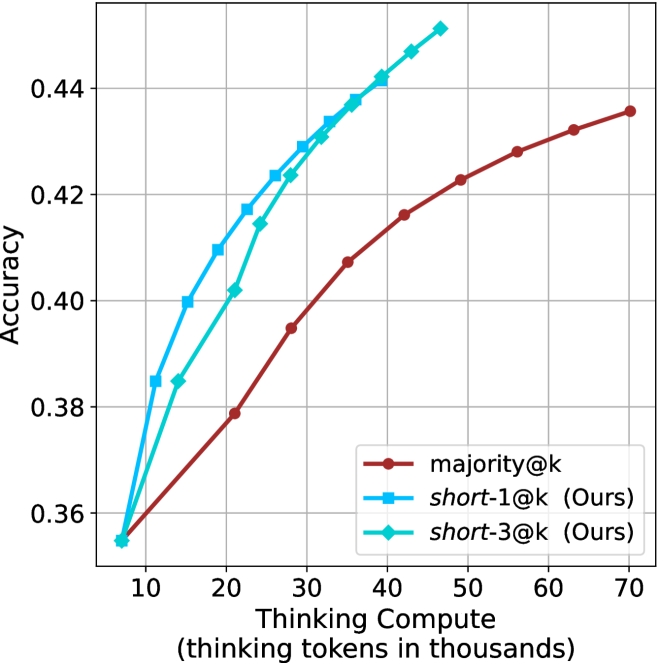
This chart illustrates the relationship between "Thinking Compute" (measured in thousands of thinking tokens) and "Accuracy" for three different methods. It compares a baseline method, `majority@k`, against two proposed methods, `short-1@k (Ours)` and `short-3@k (Ours)`. The chart demonstrates that the proposed methods achieve higher accuracy with significantly less computational expenditure compared to the baseline.
### Components/Axes
* **Y-Axis (Vertical):** Labeled "Accuracy". The scale ranges from 0.36 to 0.44, with major grid lines at 0.02 intervals.
* **X-Axis (Horizontal):** Labeled "Thinking Compute (thinking tokens in thousands)". The scale ranges from 10 to 70, with major grid lines at 10-unit intervals.
* **Legend:** Located in the bottom-right quadrant of the chart.
* `majority@k`: Represented by a dark red line with circular markers.
* `short-1@k (Ours)`: Represented by a blue line with square markers.
* `short-3@k (Ours)`: Represented by a cyan/teal line with diamond markers.
### Detailed Analysis
**Trend Verification:**
* **Common Origin:** All three data series originate from a common point at approximately (7, 0.355).
* **`majority@k` (Dark Red):** This line exhibits a steady, concave-downward slope. It is the most gradual of the three, showing a consistent increase in accuracy as compute increases, extending to the full range of the x-axis (70k tokens).
* **`short-1@k (Ours)` (Blue):** This line exhibits a sharp upward slope initially, indicating high efficiency in gaining accuracy per token. It begins to flatten (plateau) as it approaches 46k tokens.
* **`short-3@k (Ours)` (Cyan):** This line follows a trajectory very similar to `short-1@k`. It also exhibits a sharp initial slope followed by a flattening trend, terminating at approximately 47k tokens.
**Data Points (Approximate Values):**
| Thinking Compute (k) | `majority@k` (Red) | `short-1@k` (Blue) | `short-3@k` (Cyan) |
| :--- | :--- | :--- | :--- |
| ~7 | ~0.355 | ~0.355 | ~0.355 |
| 10 | ~0.362 | ~0.385 | ~0.362 |
| 15 | ~0.370 | ~0.400 | ~0.385 |
| 20 | ~0.379 | ~0.410 | ~0.402 |
| 25 | ~0.388 | ~0.417 | ~0.415 |
| 28 | ~0.395 | ~0.424 | ~0.424 |
| 35 | ~0.407 | ~0.432 | ~0.430 |
| 40 | ~0.416 | ~0.438 | ~0.438 |
| 46/47 | ~0.425 | ~0.442 | ~0.446 |
| 60 | ~0.428 | N/A | N/A |
| 70 | ~0.436 | N/A | N/A |
### Key Observations
* **Efficiency Gap:** The "Ours" methods are significantly more efficient. For instance, to reach an accuracy of ~0.42, the `majority@k` baseline requires approximately 60k tokens, whereas the `short-1@k` and `short-3@k` methods reach this level at roughly 25k–28k tokens.
* **Saturation:** The "Ours" methods appear to reach a saturation point or diminishing returns around 46k–47k tokens, where the accuracy gain per additional token becomes very small.
* **Performance:** `short-3@k` (Cyan) appears to slightly outperform `short-1@k` (Blue) in the latter half of its trajectory (post-30k tokens), reaching a higher peak accuracy before the data series ends.
### Interpretation
The data strongly suggests that the proposed "short" methods are superior to the "majority@k" baseline in terms of compute-to-accuracy efficiency. By optimizing the "thinking" process, the model can achieve higher accuracy levels with less than half the computational cost of the baseline. The fact that the "Ours" lines terminate earlier than the baseline suggests that these methods may be designed to operate within a specific, more efficient compute budget, or that they reach their maximum potential accuracy before the baseline does. This is a classic demonstration of Pareto efficiency in machine learning model optimization.