TECHNICAL ASSET FINGERPRINT
53f4983de75648a524c90671
Click to view fullscreen
Press ESC or click to close
FOUND IN PAPERS
EXPERT: gemini-2.5-flash-free VERSION 1
RUNTIME: google-free/gemini-2.5-flash
INTEL_VERIFIED
## Chart Type: Heatmap of Performance Metric
### Overview
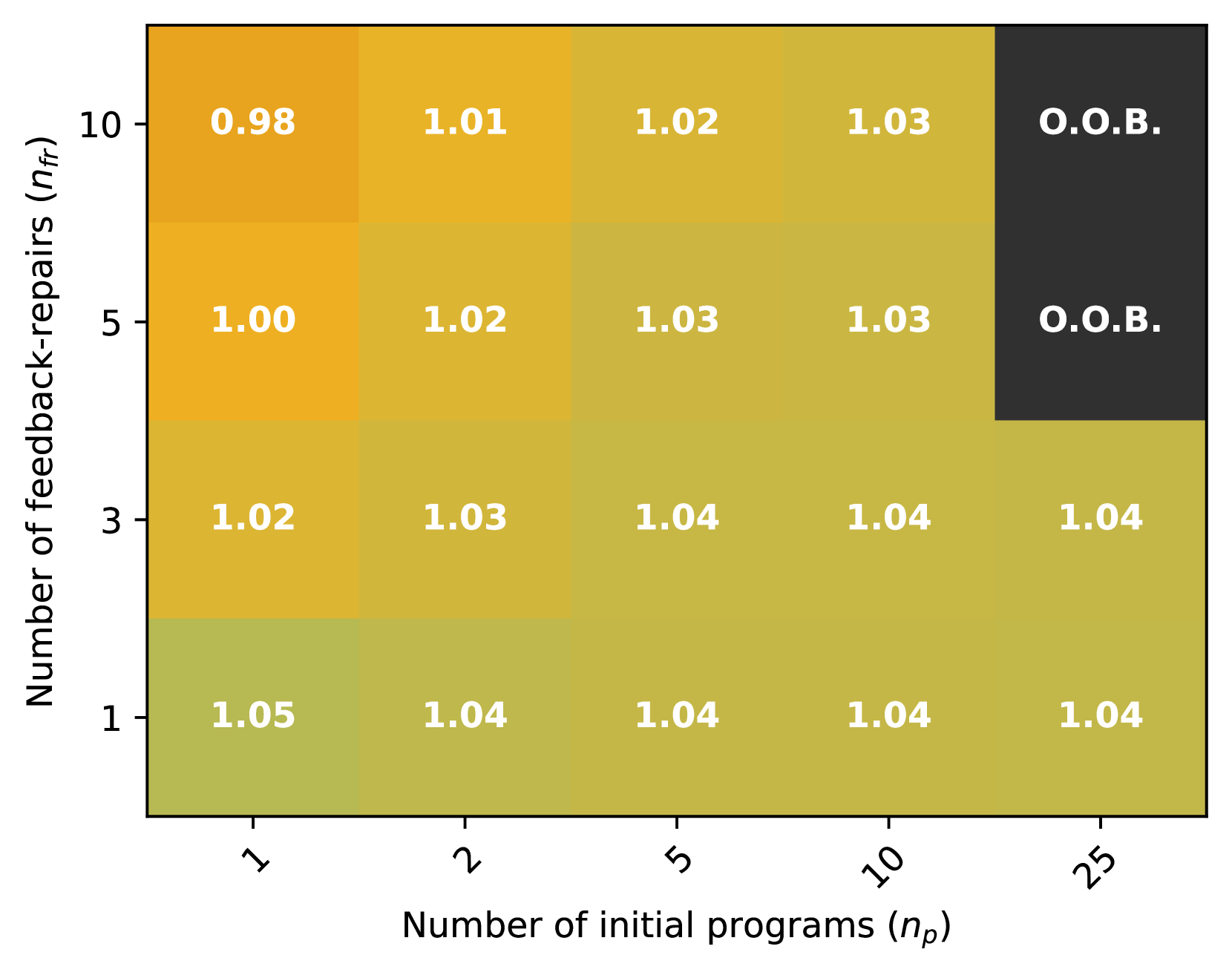
This image displays a heatmap illustrating a performance metric across varying numbers of "feedback-repairs" ($n_{fr}$) and "initial programs" ($n_p$). The grid cells contain numerical values, likely representing the performance metric, or the label "O.O.B." (Out Of Bounds). The color of the cells indicates the magnitude of the numerical value, with warmer colors (orange) generally corresponding to lower values and cooler/greener colors to higher values.
### Components/Axes
**Y-axis (Left Side):**
* **Label:** "Number of feedback-repairs ($n_{fr}$)"
* **Tick Marks (from bottom to top):** 1, 3, 5, 10
**X-axis (Bottom Side):**
* **Label:** "Number of initial programs ($n_p$)"
* **Tick Marks (from left to right):** 1, 2, 5, 10, 25
**Data Grid:**
The central area of the image is a 4x5 grid of cells. Each cell represents a unique combination of $n_{fr}$ and $n_p$ and contains a value.
**Color Gradient (Inferred - No explicit legend):**
* **Orange:** Associated with the lowest values (e.g., 0.98, 1.00, 1.01).
* **Orange-Yellow:** Associated with intermediate values (e.g., 1.02, 1.03).
* **Yellow-Green:** Associated with higher values (e.g., 1.04).
* **Green-Yellow:** Associated with the highest value (e.g., 1.05).
* **Dark Grey:** Represents "O.O.B." (Out Of Bounds).
### Detailed Analysis
The data is presented in a grid format. The rows correspond to the "Number of feedback-repairs ($n_{fr}$)" and the columns correspond to the "Number of initial programs ($n_p$)".
**Data Table:**
| $n_{fr}$ \ $n_p$ | 1 | 2 | 5 | 10 | 25 |
| :--------------- | :----- | :----- | :----- | :----- | :----- |
| **10** | 0.98 | 1.01 | 1.02 | 1.03 | O.O.B. |
| **5** | 1.00 | 1.02 | 1.03 | 1.03 | O.O.B. |
| **3** | 1.02 | 1.03 | 1.04 | 1.04 | 1.04 |
| **1** | 1.05 | 1.04 | 1.04 | 1.04 | 1.04 |
**Trends and Distributions:**
1. **Row $n_{fr}=10$ (Top Row):**
* Values start at 0.98 (orange) for $n_p=1$.
* Increase to 1.01 (orange) for $n_p=2$.
* Increase to 1.02 (orange-yellow) for $n_p=5$.
* Increase to 1.03 (orange-yellow) for $n_p=10$.
* The cell for $n_p=25$ is "O.O.B." (dark grey).
* *Trend:* Values generally increase with $n_p$ until reaching an "O.O.B." state.
2. **Row $n_{fr}=5$:**
* Values start at 1.00 (orange) for $n_p=1$.
* Increase to 1.02 (orange-yellow) for $n_p=2$.
* Increase to 1.03 (orange-yellow) for $n_p=5$.
* Remain at 1.03 (orange-yellow) for $n_p=10$.
* The cell for $n_p=25$ is "O.O.B." (dark grey).
* *Trend:* Values generally increase or stabilize with $n_p$ until reaching an "O.O.B." state.
3. **Row $n_{fr}=3$:**
* Values start at 1.02 (orange-yellow) for $n_p=1$.
* Increase to 1.03 (orange-yellow) for $n_p=2$.
* Increase to 1.04 (yellow-green) for $n_p=5$.
* Remain at 1.04 (yellow-green) for $n_p=10$.
* Remain at 1.04 (yellow-green) for $n_p=25$.
* *Trend:* Values generally increase with $n_p$ and then stabilize at 1.04.
4. **Row $n_{fr}=1$ (Bottom Row):**
* Values start at 1.05 (green-yellow) for $n_p=1$.
* Decrease to 1.04 (yellow-green) for $n_p=2$.
* Remain at 1.04 (yellow-green) for $n_p=5$.
* Remain at 1.04 (yellow-green) for $n_p=10$.
* Remain at 1.04 (yellow-green) for $n_p=25$.
* *Trend:* Values slightly decrease with $n_p$ and then stabilize at 1.04.
**Column-wise Trends:**
* **Column $n_p=1$ (Leftmost):** Values increase from 0.98 ($n_{fr}=10$) to 1.05 ($n_{fr}=1$).
* **Column $n_p=2$:** Values increase from 1.01 ($n_{fr}=10$) to 1.04 ($n_{fr}=1$).
* **Column $n_p=5$:** Values increase from 1.02 ($n_{fr}=10$) to 1.04 ($n_{fr}=1$).
* **Column $n_p=10$:** Values increase from 1.03 ($n_{fr}=10$) to 1.04 ($n_{fr}=1$).
* **Column $n_p=25$ (Rightmost):** Values are "O.O.B." for $n_{fr}=10$ and $n_{fr}=5$, then become 1.04 for $n_{fr}=3$ and $n_{fr}=1$.
### Key Observations
* **Minimum Value:** The lowest performance metric value observed is 0.98, located at $n_{fr}=10, n_p=1$. This cell is distinctly orange.
* **Maximum Value:** The highest performance metric value observed is 1.05, located at $n_{fr}=1, n_p=1$. This cell is green-yellow.
* **"O.O.B." Region:** The top-right corner of the grid, specifically for $n_p=25$ when $n_{fr}=10$ or $n_{fr}=5$, shows "O.O.B.". This indicates a region where the process or experiment was not applicable, failed, or exceeded some boundary condition.
* **Stabilization:** For lower numbers of feedback-repairs ($n_{fr}=3$ and $n_{fr}=1$), the performance metric tends to stabilize at 1.04 as the number of initial programs ($n_p$) increases.
* **Color-Value Relationship:** The color scheme suggests that lower numerical values (closer to 0.98) are "better" or more desirable, as they are represented by a distinct orange, while higher values (closer to 1.05) are represented by greener hues.
### Interpretation
This heatmap likely represents the outcome of an experiment or simulation where the "Number of feedback-repairs ($n_{fr}$)" and "Number of initial programs ($n_p$)" are input parameters, and the numerical values in the cells are a measure of system performance or efficiency.
The inverse relationship between color and value (orange for low, green for high) suggests that the metric being measured is one where lower values are more favorable. For example, it could be an error rate, a cost, or a time taken.
The data suggests that:
1. **Optimal Performance:** The best performance (0.98) is achieved when there is a high number of feedback-repairs ($n_{fr}=10$) and a minimal number of initial programs ($n_p=1$). This implies that extensive refinement (feedback-repairs) on a single or very few initial attempts is most effective under these conditions.
2. **Impact of Initial Programs:** Generally, increasing the "Number of initial programs ($n_p$)" tends to degrade performance (increase the metric value) or lead to an "Out Of Bounds" state, especially when combined with a high number of feedback-repairs. This could mean that too many initial programs introduce complexity or redundancy that hinders the process, or that the system struggles to manage a large pool of initial programs with many feedback loops.
3. **Impact of Feedback-Repairs:** Decreasing the "Number of feedback-repairs ($n_{fr}$)" generally leads to worse performance (higher metric values). This highlights the importance of feedback and repair mechanisms for achieving better outcomes.
4. **System Limitations ("O.O.B."):** The "O.O.B." cells in the top-right corner indicate a boundary condition. It's plausible that running a high number of feedback-repairs on a large number of initial programs is computationally too expensive, leads to resource exhaustion, or simply falls outside the defined scope of the experiment. For example, if $n_p$ represents parallel processes and $n_{fr}$ represents iterations, a high combination might exceed available processing power or time limits.
5. **Convergence:** For lower $n_{fr}$ values (1 and 3), the performance metric seems to converge to 1.04 regardless of the number of initial programs (beyond $n_p=2$). This suggests a baseline performance level that cannot be significantly improved by adding more initial programs if feedback-repairs are limited.
In essence, the data points to a trade-off: while a high number of feedback-repairs is beneficial, it needs to be balanced with a relatively low number of initial programs to achieve optimal results and avoid "out of bounds" scenarios. The sweet spot for this particular metric appears to be at the lowest $n_p$ and highest $n_{fr}$ tested.
DECODING INTELLIGENCE...