## Line Graph: Accuracy vs. Time with Hyperparameter Variations
### Overview
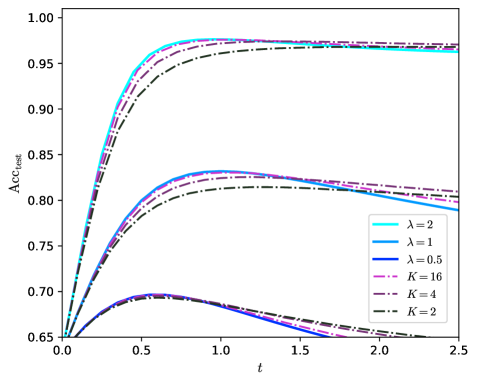
The image is a line graph comparing the test accuracy (Acc_test) of a model over time (t) under different hyperparameter configurations. Two y-axes are present: the left axis represents accuracy (0.65–1.00), and the right axis represents time (0.0–2.5). The graph includes six data series differentiated by line style and color, corresponding to combinations of λ (learning rate) and K (number of components).
### Components/Axes
- **X-axis (t)**: Time, ranging from 0.0 to 2.5.
- **Left Y-axis (Acc_test)**: Test accuracy, ranging from 0.65 to 1.00.
- **Right Y-axis (t)**: Time, ranging from 0.0 to 2.5 (duplicate of x-axis, likely for reference).
- **Legend**: Located in the bottom-right corner, mapping:
- **λ values**:
- Cyan (solid): λ = 2
- Blue (solid): λ = 1
- Dark blue (solid): λ = 0.5
- **K values**:
- Magenta (dashed): K = 16
- Purple (dash-dot): K = 4
- Black (dotted): K = 2
### Detailed Analysis
1. **λ = 2 (Cyan Solid Line)**:
- Starts at 0.65 at t=0.0.
- Rises sharply to ~0.95 by t=0.5.
- Plateaus near 0.95 for t > 0.5.
- **Trend**: Fastest initial improvement, stable at high accuracy.
2. **λ = 1 (Blue Solid Line)**:
- Starts at 0.65 at t=0.0.
- Rises to ~0.93 by t=0.5.
- Slightly declines to ~0.92 by t=2.5.
- **Trend**: Moderate improvement, minor decline over time.
3. **λ = 0.5 (Dark Blue Solid Line)**:
- Starts at 0.65 at t=0.0.
- Rises slowly to ~0.88 by t=0.5.
- Declines to ~0.85 by t=2.5.
- **Trend**: Slowest improvement, gradual decline.
4. **K = 16 (Magenta Dashed Line)**:
- Starts at 0.65 at t=0.0.
- Peaks at ~0.95 by t=0.5.
- Declines to ~0.90 by t=2.5.
- **Trend**: Highest peak but significant drop after t=0.5.
5. **K = 4 (Purple Dash-Dot Line)**:
- Starts at 0.65 at t=0.0.
- Rises to ~0.92 by t=0.5.
- Declines to ~0.89 by t=2.5.
- **Trend**: Balanced improvement and decline.
6. **K = 2 (Black Dotted Line)**:
- Starts at 0.65 at t=0.0.
- Rises to ~0.85 by t=0.5.
- Declines to ~0.83 by t=2.5.
- **Trend**: Lowest performance, steady decline.
### Key Observations
- **λ vs. K Trade-off**: Higher λ values (2, 1) achieve higher accuracy than lower λ (0.5), but K=16 (magenta) initially outperforms all λ values.
- **Temporal Decline**: All lines show a decline after t=0.5, suggesting potential overfitting or parameter sensitivity over time.
- **K=16 Anomaly**: Despite the highest peak, K=16 experiences the steepest decline, indicating possible instability at high K values.
### Interpretation
The graph demonstrates that **higher λ values (2, 1)** yield better sustained accuracy compared to lower λ (0.5), but **K=16** achieves the highest initial accuracy. However, the sharp decline in K=16’s performance after t=0.5 suggests that increasing K may lead to overfitting or instability. The consistent decline across all lines after t=0.5 implies that the model’s performance degrades over time, possibly due to data drift or parameter tuning requirements. The interplay between λ and K highlights the need for careful hyperparameter optimization to balance initial gains with long-term stability.