## Diagram: Auditory Signal Processing Pipeline and Frequency Response Analysis
### Overview
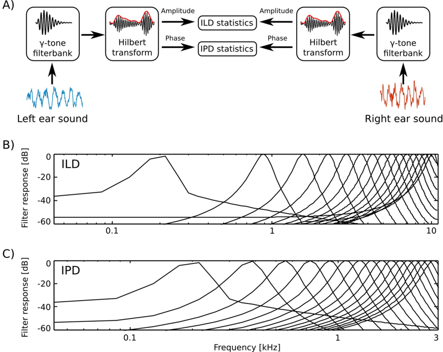
The image presents a technical diagram of a binaural auditory signal processing system, combining signal transformation workflows (Part A) with frequency response graphs for Interaural Level Differences (ILD) and Interaural Phase Differences (IPD) (Parts B and C). The system processes left/right ear sounds through filterbanks, Hilbert transforms, and statistical analysis to model spatial hearing cues.
---
### Components/Axes
#### Part A: Signal Processing Workflow
1. **Left Ear Path**:
- Input: "Left ear sound" (blue waveform)
- Components:
- `y-tone filterbank` → `Hilbert transform` → `Amplitude` → `ILD statistics`
- `Phase` → `IPD statistics`
2. **Right Ear Path**:
- Input: "Right ear sound" (red waveform)
- Components:
- `y-tone filterbank` → `Hilbert transform` → `Amplitude` → `ILD statistics`
- `Phase` → `IPD statistics`
3. **Key Elements**:
- Arrows indicate signal flow direction
- Red/blue waveforms distinguish left/right ear inputs
- Hilbert transform outputs are highlighted in red
#### Part B: ILD Frequency Response
- **Axes**:
- X-axis: Frequency (kHz), logarithmic scale (0.1 to 10 kHz)
- Y-axis: Filter response (dB), linear scale (-60 to 0 dB)
- **Legend**: No explicit legend; lines represent multiple frequency response curves
#### Part C: IPD Frequency Response
- **Axes**:
- X-axis: Frequency (kHz), logarithmic scale (0.1 to 3 kHz)
- Y-axis: Filter response (dB), linear scale (-60 to 0 dB)
- **Legend**: No explicit legend; lines represent multiple frequency response curves
---
### Detailed Analysis
#### Part A: Signal Processing Flow
1. **Left Ear**:
- Blue waveform enters `y-tone filterbank`, splitting into amplitude/phase components.
- Amplitude → `ILD statistics` (interaural level differences).
- Phase → `IPD statistics` (interaural phase differences).
2. **Right Ear**:
- Red waveform follows identical processing steps but with distinct Hilbert transform output.
- Amplitude/phase data from both ears are compared to compute ILD/IPD.
#### Part B: ILD Frequency Response
- **Trends**:
- Multiple curves show filter responses peaking at ~1 kHz (highest amplitude).
- Responses decline sharply above 10 kHz.
- Lower frequencies (<0.1 kHz) exhibit minimal filtering.
- **Notable Features**:
- Curves exhibit "notch" patterns at mid-frequencies (1–10 kHz), suggesting bandpass filtering.
#### Part C: IPD Frequency Response
- **Trends**:
- Peaks occur at ~0.1 kHz (low-frequency dominance).
- Responses diminish above 1 kHz, with near-zero filtering beyond 3 kHz.
- Mid-frequency ranges (0.5–2 kHz) show moderate filtering.
---
### Key Observations
1. **ILD vs. IPD Frequency Sensitivity**:
- ILD is most sensitive to mid/high frequencies (1–10 kHz).
- IPD is most sensitive to low frequencies (0.1–1 kHz).
2. **Symmetry in Processing**:
- Both ears use identical processing steps, emphasizing binaural comparison.
3. **Waveform Differences**:
- Left ear (blue) and right ear (red) waveforms differ in amplitude/phase, critical for spatial localization.
---
### Interpretation
This system models how humans localize sound sources using ILD and IPD. The frequency-dependent filtering in Parts B and C reflects the human auditory system's reliance on:
- **ILD** for high-frequency sound localization (e.g., speech consonants).
- **IPD** for low-frequency sound localization (e.g., vowel formants).
The Hilbert transform in Part A extracts instantaneous amplitude/phase data, enabling precise statistical analysis of interaural differences. The absence of a legend in Parts B/C suggests the curves represent a range of filter settings or experimental conditions, requiring further context for interpretation.