\n
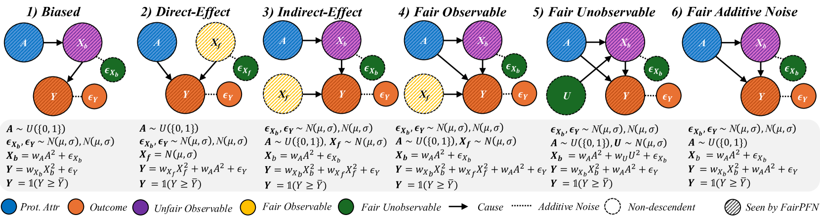
## Diagram: Fairness Scenarios in Machine Learning
### Overview
The image presents a series of six diagrams illustrating different scenarios related to fairness in machine learning models. Each scenario depicts a causal diagram with nodes representing protected attributes, unfair observable features, fair observable features, outcomes, and error terms. The diagrams aim to visualize how different types of bias and unfairness can manifest in a model's decision-making process.
### Components/Axes
The diagrams share the following components:
* **Protected Attribute (Prot. Attr):** Represented by a teal-colored circle labeled "A".
* **Outcome:** Represented by a purple circle labeled "Y".
* **Unfair Observable:** Represented by an orange circle labeled "X<sub>b</sub>".
* **Fair Observable:** Represented by a yellow circle labeled "X<sub>f</sub>".
* **Error Terms:** Represented by small, light-blue circles labeled "ε<sub>x</sub>" and "ε<sub>y</sub>".
* **Arrows:** Indicate causal relationships between variables.
* **Legend:** Located at the bottom-right, defining the color-coding for each component.
* **Mathematical Equations:** Below each diagram, defining the relationships between variables.
* **Titles:** Above each diagram, indicating the fairness scenario (1) Biased, (2) Direct-Effect, (3) Indirect-Effect, (4) Fair Observable, (5) Fair Unobservable, (6) Fair Additive Noise.
### Content Details
Here's a breakdown of each scenario, including the equations:
**1) Biased:**
* A -> X<sub>b</sub> -> Y
* A -> X<sub>f</sub> -> Y
* Equation: A ~ U(0,1), ε<sub>x</sub>, ε<sub>y</sub> ~ N(μ,0), σ, X<sub>b</sub> = W<sub>A</sub><sup>2</sup> + ε<sub>x</sub>, X<sub>f</sub> = W<sub>A</sub><sup>2</sup> + ε<sub>x</sub>, Y = W<sub>x</sub>X<sub>b</sub> + W<sub>x</sub>X<sub>f</sub> + ε<sub>y</sub>, Y = 1(Y ≥ γ)
**2) Direct-Effect:**
* A -> X<sub>b</sub> -> Y
* A -> X<sub>f</sub>
* Equation: A ~ U(0,1), X<sub>b</sub> ~ N(μ<sub>A</sub>,0), X<sub>f</sub> ~ N(μ<sub>0</sub>,0), X<sub>f</sub> = N(μ<sub>0</sub>), Y = W<sub>x</sub>X<sub>b</sub> + W<sub>x</sub>X<sub>f</sub> + ε<sub>y</sub>, Y = 1(Y ≥ γ)
**3) Indirect-Effect:**
* A -> X<sub>f</sub> -> X<sub>b</sub> -> Y
* Equation: ε<sub>x</sub>, ε<sub>y</sub> ~ N(μ,0), A ~ U(0,1), X<sub>f</sub> ~ N(μ<sub>0</sub>), X<sub>b</sub> = W<sub>A</sub><sup>2</sup> + ε<sub>x</sub>, Y = W<sub>x</sub>X<sub>b</sub> + W<sub>x</sub>X<sub>f</sub> + ε<sub>y</sub>, Y = 1(Y ≥ γ)
**4) Fair Observable:**
* A -> X<sub>f</sub> -> Y
* Equation: ε<sub>x</sub>, ε<sub>y</sub> ~ N(μ,0), A ~ U(0,1), X<sub>f</sub> ~ N(μ<sub>0</sub>), X<sub>b</sub> = W<sub>A</sub><sup>2</sup> + ε<sub>x</sub>, Y = W<sub>x</sub>X<sub>b</sub> + W<sub>x</sub>X<sub>f</sub> + ε<sub>y</sub>, Y = 1(Y ≥ γ)
**5) Fair Unobservable:**
* A -> U -> X<sub>b</sub> -> Y
* Equation: ε<sub>x</sub>, ε<sub>y</sub> ~ N(μ,0), A ~ U(0,1), U ~ N(μ<sub>0</sub>), X<sub>b</sub> = W<sub>A</sub><sup>2</sup> + W<sub>U</sub><sup>1</sup> + ε<sub>x</sub>, Y = W<sub>x</sub>X<sub>b</sub> + W<sub>x</sub>X<sub>f</sub> + ε<sub>y</sub>, Y = 1(Y ≥ γ)
**6) Fair Additive Noise:**
* A -> X<sub>b</sub> -> Y
* Equation: ε<sub>x</sub>, ε<sub>y</sub> ~ N(μ,0), A ~ U(0,1), X<sub>b</sub> = W<sub>A</sub><sup>2</sup> + ε<sub>x</sub>, X<sub>f</sub> = W<sub>A</sub><sup>2</sup> + ε<sub>x</sub>, Y = W<sub>x</sub>X<sub>b</sub> + W<sub>x</sub>X<sub>f</sub> + ε<sub>y</sub>, Y = 1(Y ≥ γ)
### Key Observations
* The diagrams consistently use the same node representations and causal arrow style.
* The mathematical equations provide a formal definition of the relationships depicted in each diagram.
* The scenarios vary in how the protected attribute (A) influences the outcome (Y), either directly, indirectly, or through observable/unobservable features.
* The inclusion of error terms (ε<sub>x</sub>, ε<sub>y</sub>) acknowledges the inherent noise and uncertainty in real-world data.
* The use of U(0,1) indicates a uniform distribution, while N(μ,σ) indicates a normal distribution.
### Interpretation
These diagrams illustrate different ways in which bias can enter a machine learning model and affect its fairness. They highlight the importance of considering causal relationships when evaluating and mitigating bias.
* **Scenario 1 (Biased):** Demonstrates a simple case where the protected attribute directly influences both observable features and the outcome, leading to potential discrimination.
* **Scenario 2 (Direct-Effect):** Shows a direct causal link between the protected attribute and the outcome, bypassing observable features.
* **Scenario 3 (Indirect-Effect):** Illustrates how the protected attribute can indirectly influence the outcome through a fair observable feature.
* **Scenario 4 (Fair Observable):** Suggests a scenario where fairness is achieved by ensuring that the observable features are independent of the protected attribute.
* **Scenario 5 (Fair Unobservable):** Introduces an unobservable variable (U) that mediates the relationship between the protected attribute and the outcome.
* **Scenario 6 (Fair Additive Noise):** Represents a scenario where fairness is achieved by adding noise to the model's predictions.
The diagrams, combined with the mathematical equations, provide a rigorous framework for analyzing and addressing fairness concerns in machine learning. They emphasize the need to understand the underlying causal mechanisms that drive bias and to develop interventions that target those mechanisms effectively. The "Seen by FairPFN" label at the bottom right suggests these diagrams are related to a specific fairness-aware machine learning framework or algorithm.