TECHNICAL ASSET FINGERPRINT
59f1f0360ad7a95a7eeeeae4
Click to view fullscreen
Press ESC or click to close
FOUND IN PAPERS
EXPERT: healer-alpha-free VERSION 1
RUNTIME: free/openrouter/healer-alpha
INTEL_VERIFIED
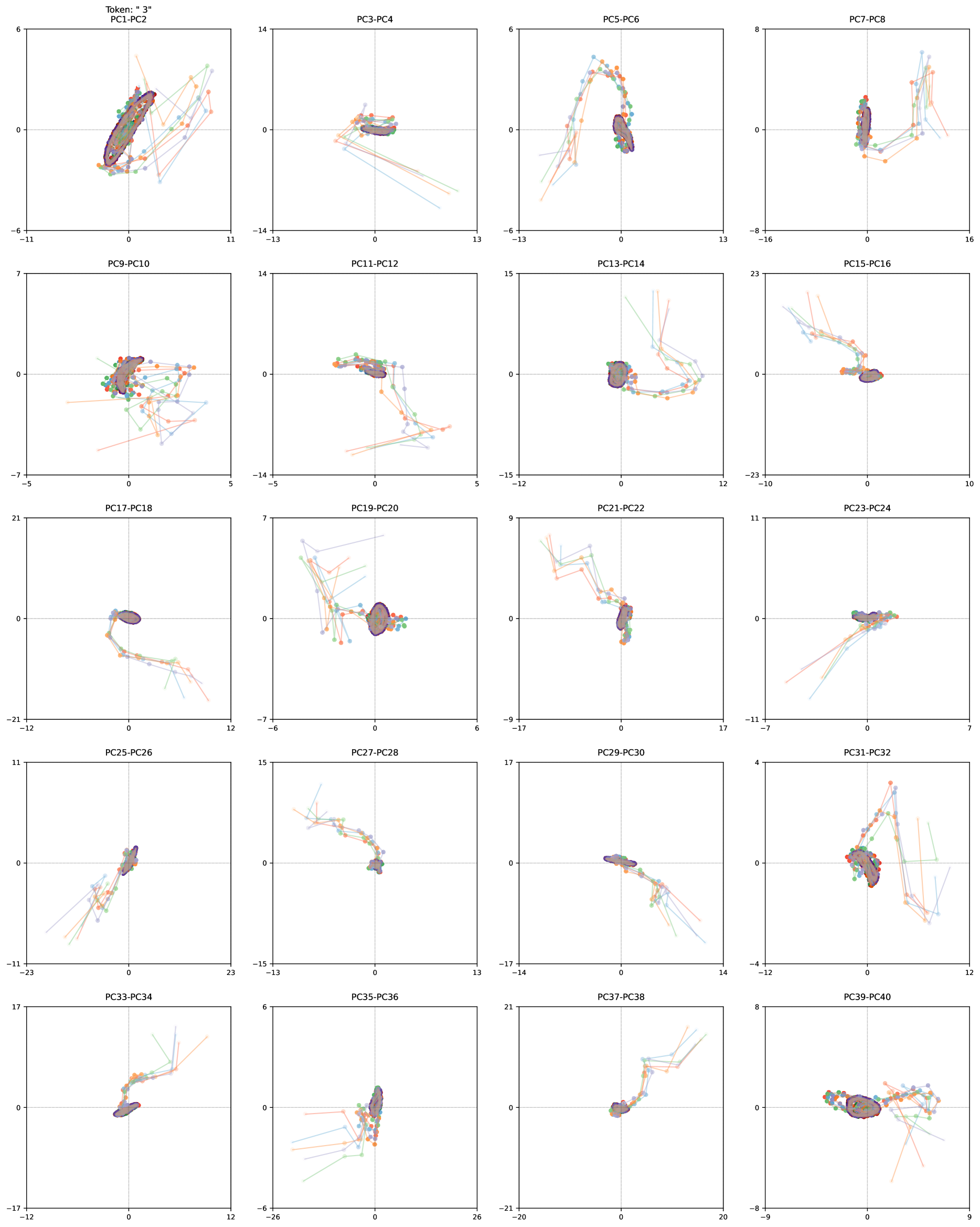
## Scatter Plot Grid: Principal Component Analysis (PCA) Projections for Token "3"
### Overview
The image displays a 5x4 grid of 20 scatter plots, each visualizing the relationship between pairs of principal components (PCs). The overall title at the top-left corner is **Token: "3"**. Each subplot represents a 2D projection of data onto a specific pair of principal components (e.g., PC1 vs. PC2, PC3 vs. PC4, etc.), likely from a high-dimensional dataset related to the token "3". The data points are colored in multiple hues (orange, green, blue, purple, etc.) and are connected by faint lines, suggesting trajectories or sequences across the principal component space.
### Components/Axes
* **Global Title:** `Token: "3"` (Top-left corner of the entire figure).
* **Subplot Grid:** 5 rows by 4 columns.
* **Subplot Titles:** Each subplot is titled with its corresponding PC pair (e.g., `PC1-PC2`, `PC3-PC4`, ..., `PC39-PC40`).
* **Axes:** Each subplot has an x-axis and a y-axis representing the values of the respective principal components. The axis scales (ranges) vary significantly between subplots.
* **Data Series:** Multiple colored series (points connected by lines) are present in each plot. The colors observed include orange, green, light blue, dark blue, and purple. There is no explicit legend provided within the image to define what each color represents.
### Detailed Analysis
Below is a plot-by-plot analysis, noting axis ranges and the general visual trend of the data points. The colors are described based on visual inspection (e.g., orange, green, blue, purple).
**Row 1:**
1. **PC1-PC2:** X: [-11, 11], Y: [-6, 6]. Data forms a dense, elongated cluster oriented diagonally from bottom-left to top-right, centered near (0,0). Multiple colored trajectories are visible.
2. **PC3-PC4:** X: [-13, 13], Y: [-14, 14]. A tight cluster near (0,0) with several long, linear trajectories extending primarily towards the bottom-right quadrant.
3. **PC5-PC6:** X: [-13, 13], Y: [-6, 6]. Data forms a distinct inverted "U" or arch shape, peaking around Y=4. The cluster is dense at the right end of the arch.
4. **PC7-PC8:** X: [-16, 16], Y: [-8, 8]. A dense vertical cluster near X=0, with several trajectories extending to the right and slightly upward.
**Row 2:**
5. **PC9-PC10:** X: [-5, 5], Y: [-7, 7]. A central cluster with trajectories spreading out in multiple directions, particularly to the left and bottom.
6. **PC11-PC12:** X: [-5, 5], Y: [-14, 14]. A cluster near the origin with long, downward-sloping trajectories extending to the bottom-right.
7. **PC13-PC14:** X: [-12, 12], Y: [-15, 15]. A cluster near (0,0) with trajectories forming a loose, downward-curving shape to the right.
8. **PC15-PC16:** X: [-10, 10], Y: [-23, 23]. A dense cluster near the origin with a few long, linear trajectories extending to the top-left.
**Row 3:**
9. **PC17-PC18:** X: [-12, 12], Y: [-21, 21]. A cluster near the origin with trajectories extending downward and to the right.
10. **PC19-PC20:** X: [-6, 6], Y: [-7, 7]. A dense cluster near (0,0) with several trajectories spreading out, notably to the top-left.
11. **PC21-PC22:** X: [-17, 17], Y: [-9, 9]. A cluster near the origin with trajectories extending upward and to the left.
12. **PC23-PC24:** X: [-7, 7], Y: [-11, 11]. A tight horizontal cluster near Y=0, with trajectories extending to the bottom-left.
**Row 4:**
13. **PC25-PC26:** X: [-23, 23], Y: [-11, 11]. A cluster near the origin with trajectories extending to the bottom-left.
14. **PC27-PC28:** X: [-13, 13], Y: [-15, 15]. A cluster near the origin with trajectories extending to the top-left.
15. **PC29-PC30:** X: [-14, 14], Y: [-17, 17]. A cluster near the origin with trajectories extending to the bottom-right.
16. **PC31-PC32:** X: [-12, 12], Y: [-4, 4]. A dense cluster near the origin with trajectories forming a loop or upward curve to the right.
**Row 5:**
17. **PC33-PC34:** X: [-12, 12], Y: [-17, 17]. A cluster near the origin with trajectories extending to the top-right.
18. **PC35-PC36:** X: [-26, 26], Y: [-6, 6]. A cluster near the origin with trajectories extending to the bottom-left.
19. **PC37-PC38:** X: [-20, 20], Y: [-21, 21]. A cluster near the origin with trajectories extending to the top-right.
20. **PC39-PC40:** X: [-9, 9], Y: [-8, 8]. A cluster near the origin with trajectories spreading out, notably to the right.
### Key Observations
1. **Common Structure:** Nearly all plots show a dense core cluster of points centered at or near the origin (0,0), with various trajectories or "arms" extending outward. This suggests the data has a central tendency with directional variations captured by different PC pairs.
2. **Variable Spread:** The scale of the axes varies dramatically (e.g., PC15-PC16 Y-axis spans 46 units, while PC31-PC32 Y-axis spans only 8 units). This indicates that the variance explained by each principal component pair is not uniform.
3. **Distinct Shapes:** Some PC pairs reveal clear geometric patterns:
* **Arch/Inverted U:** PC5-PC6.
* **Vertical/Horizontal Clusters:** PC7-PC8 (vertical), PC23-PC24 (horizontal).
* **Diagonal Orientation:** PC1-PC2.
4. **Trajectory Direction:** The direction of the extending trajectories (e.g., top-left, bottom-right) is specific to each PC pair, indicating the axes of variation in the high-dimensional space.
5. **Color Patterns:** The same color (e.g., orange, green) appears to follow consistent trajectories within a given plot, suggesting the colors represent distinct classes, sequences, or experimental conditions that evolve through the PC space.
### Interpretation
This grid of scatter plots is a diagnostic visualization from a Principal Component Analysis (PCA) performed on data associated with the token "3". PCA is a dimensionality reduction technique used to visualize high-dimensional data in lower dimensions (here, 2D) while preserving as much variance as possible.
* **What the data suggests:** The consistent central cluster with radiating trajectories implies that the underlying data for token "3" has a stable "core" representation, but also exhibits systematic variations or modes of change. Each PC pair captures a different axis of this variation. For example, the arch in PC5-PC6 might represent a continuous transformation or cycle in the data.
* **How elements relate:** The 20 plots are complementary views of the same high-dimensional dataset. A point's position in one plot (e.g., PC1-PC2) is independent of its position in another (e.g., PC3-PC4), but together they provide a more complete picture of the data's structure. The colored trajectories likely track the same data points (or groups) across different projection planes.
* **Notable anomalies/trends:** The most striking features are the non-random, structured shapes (arches, lines, clusters). This indicates the data is not noise but has meaningful, low-dimensional structure. The fact that trajectories are often linear or smoothly curved suggests the variations are orderly. The lack of scattered, random points reinforces that the token "3" has a well-defined representation in this feature space.
* **Purpose:** This type of analysis is common in machine learning and natural language processing to understand the internal representations of tokens in a model. It helps researchers see if different contexts or uses of the same token ("3") cluster together or separate in the model's latent space, and what the primary directions of variation are.
DECODING INTELLIGENCE...