## Chart: Distribution Plot ### Overview The image shows a distribution plot with two overlapping curves, one blue and one orange. The plot visualizes the distribution of some variable, with the x-axis ranging from approximately -1.5 to 0.5 and the y-axis representing the density or frequency of the variable. ### Components/Axes * **X-axis:** Ranges from -1.5 to 0.5, with tick marks at -1.5, -1.0, -0.5, 0.0, and 0.5. * **Y-axis:** Ranges from 0 to approximately 7, with tick marks at 0, 2, 4, and 6. * **Blue Curve:** Represents one distribution. * **Orange Curve:** Represents another distribution. ### Detailed Analysis * **Blue Curve:** The blue curve starts near 0 at x = -1.5, gradually increases to a peak around x = 0.25 with a y-value of approximately 1.5, and then decreases back to near 0 at x = 0.5. * **Orange Curve:** The orange curve starts near 0 at x = -1.5, increases to a peak around x = -0.3 with a y-value of approximately 1.8, and then decreases back to near 0 at x = 0.5. ### Key Observations * The orange curve is shifted to the left compared to the blue curve. * Both curves are unimodal, meaning they have a single peak. * The peak of the orange curve is slightly higher than the peak of the blue curve. * The blue curve appears to be slightly wider than the orange curve, indicating a larger standard deviation. ### Interpretation The plot compares the distributions of two different variables or groups. The orange distribution has a lower mean than the blue distribution, as indicated by its peak being shifted to the left. The blue distribution has a slightly larger spread, suggesting greater variability. The difference in the distributions could be due to various factors depending on the context of the data.

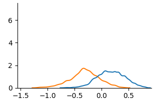
\n ## Chart: Density Plot ### Overview The image displays a density plot with two overlapping curves. The x-axis ranges from -1.5 to 0.5, and the y-axis ranges from 0 to 6. The plot appears to represent the distribution of two datasets. ### Components/Axes * **X-axis:** Labeled with numerical values from -1.5 to 0.5, with tick marks at -1.0, -0.5, and 0.0. * **Y-axis:** Labeled with numerical values from 0 to 6, with tick marks at 0, 2, 4, and 6. * **Curve 1 (Orange):** Represents one dataset's distribution. * **Curve 2 (Blue):** Represents another dataset's distribution. * **No Legend:** There is no explicit legend identifying the datasets represented by each curve. ### Detailed Analysis * **Curve 1 (Orange):** This curve starts at approximately y=0 at x=-1.5. It gradually increases, reaching a peak of approximately y=2 at x=-0.5. It then decreases, crossing y=0 around x=0.2. The curve is unimodal. * **Curve 2 (Blue):** This curve starts at approximately y=0 at x=-1.5. It increases more rapidly than the orange curve, reaching a peak of approximately y=1.7 at x=-0.2. It then decreases, with a slight plateau around x=0.1, and crosses y=0 around x=0.4. The curve is also unimodal. * **Overlap:** The two curves overlap significantly between x=-0.5 and x=0.2. The blue curve is generally higher than the orange curve in this region. * **Data Points (Approximate):** * Orange Curve: (-1.5, 0), (-1.0, 0.2), (-0.5, 2.0), (0.0, 0.8), (0.2, 0.0) * Blue Curve: (-1.5, 0), (-1.0, 0.5), (-0.5, 1.2), (-0.2, 1.7), (0.0, 1.0), (0.2, 0.5), (0.4, 0.0) ### Key Observations * Both datasets appear to be similarly distributed, with a slight skew towards positive values. * The blue dataset has a higher peak and is generally more concentrated around x=-0.2. * The orange dataset is more spread out and has a peak at x=-0.5. ### Interpretation The chart suggests that the two datasets represent distributions with similar shapes but different central tendencies. The blue dataset is shifted slightly to the right compared to the orange dataset, indicating a higher average value. The overlap between the curves suggests that there is some commonality between the two datasets, but they are not identical. Without knowing what these datasets represent, it's difficult to draw more specific conclusions. The lack of a legend makes it impossible to determine what the curves represent. The chart could be visualizing the distribution of two different populations, or the distribution of a single variable before and after some intervention. The data suggests a possible difference in the underlying processes generating these distributions.

## Line Chart: Dual Distribution Curves ### Overview The image displays a 2D line chart featuring two smooth, bell-shaped curves plotted against a common horizontal axis. The chart lacks a title, axis labels, and a legend, presenting only the numerical scales and the plotted data series. The visual suggests a comparison between two related distributions or functions. ### Components/Axes * **X-Axis (Horizontal):** * **Scale:** Linear. * **Range:** Approximately -1.5 to 0.5. * **Major Tick Marks & Labels:** Located at -1.5, -1.0, -0.5, 0.0, 0.5. * **Y-Axis (Vertical):** * **Scale:** Linear. * **Range:** 0 to 6. * **Major Tick Marks & Labels:** Located at 0, 2, 4, 6. * **Data Series:** * **Series 1 (Blue Line):** A smooth, unimodal curve. * **Series 2 (Orange Line):** A smooth, unimodal curve. * **Legend:** **Not present.** The identity and meaning of the blue and orange lines are not defined within the image. ### Detailed Analysis * **Blue Curve Trend & Points:** * **Trend:** The curve starts near y=0 at the far left (x ≈ -1.5), rises gradually, accelerates to a peak, then descends symmetrically. * **Key Points (Approximate):** * Start: (x ≈ -1.5, y ≈ 0) * Peak: (x ≈ 0.2, y ≈ 1.5) * End: (x ≈ 0.5, y ≈ 0) * **Orange Curve Trend & Points:** * **Trend:** The curve starts near y=0 at the far left (x ≈ -1.5), rises more steeply than the blue curve to an earlier peak, then descends. * **Key Points (Approximate):** * Start: (x ≈ -1.5, y ≈ 0) * Peak: (x ≈ -0.3, y ≈ 2.0) * End: (x ≈ 0.5, y ≈ 0) * **Spatial Relationship:** The orange curve is positioned to the left of and reaches a higher maximum value than the blue curve. The two curves intersect at approximately (x ≈ -0.05, y ≈ 1.0). ### Key Observations 1. **Missing Context:** The most significant observation is the complete absence of explanatory labels (chart title, axis titles, legend). This renders the chart's specific subject matter and the identity of the two series unknown. 2. **Distribution Shapes:** Both curves resemble probability density functions (e.g., Gaussian/Normal distributions) or similar mathematical functions, characterized by their smooth, symmetric, bell-like shapes. 3. **Comparative Properties:** The orange distribution has a **higher peak** (mode) and a **lower mean** (centered further left on the x-axis) compared to the blue distribution. The blue distribution appears slightly wider (larger variance/spread). 4. **Data Range:** The meaningful data for both series is concentrated between x = -1.0 and x = 0.5. ### Interpretation The chart visually compares two distinct but related quantitative distributions. The lack of labels forces a purely formal interpretation: * **What it demonstrates:** It shows two unimodal datasets or functions where one (orange) is centered on a lower value of the measured variable (x-axis) and has a higher concentration of values near its center (higher peak) than the other (blue). * **How elements relate:** The x-axis represents a continuous independent variable. The y-axis represents a dependent variable, likely frequency, probability density, or magnitude. The curves show how this dependent variable changes across the range of the independent variable for two different groups, conditions, or models. * **Potential Contexts (Speculative):** Without labels, this could represent: * Comparison of two sensor readings or signal distributions. * Results from two different statistical models or machine learning algorithms. * Performance metrics under two different conditions. * Physical measurements of two similar phenomena. * **Notable Anomaly:** The primary anomaly is the chart's lack of self-contained explanatory information, which is a critical flaw for a technical document. The data is presented without the necessary context for meaningful analysis. **Language Note:** No non-English text is present in the image.

## Line Graph: Unlabeled Data Series Comparison ### Overview The image depicts a line graph with two distinct data series represented by orange and blue lines. The x-axis spans from -1.5 to 0.5, while the y-axis ranges from 0 to 6. Both lines exhibit unimodal distributions with peaks in the negative and positive x-regions, respectively. The graph lacks explicit axis labels, titles, or contextual annotations. ### Components/Axes - **X-Axis**: Labeled with numerical values from -1.5 to 0.5 in increments of 0.5. No explicit label text is visible. - **Y-Axis**: Labeled with numerical values from 0 to 6 in increments of 2. No explicit label text is visible. - **Legend**: Located in the top-right corner, associating: - **Orange line**: "Line A" - **Blue line**: "Line B" ### Detailed Analysis 1. **Orange Line (Line A)**: - **Trend**: Starts near zero at x ≈ -1.5, rises gradually to a peak at x ≈ -0.5 (y ≈ 1.8), then declines sharply to near zero by x ≈ 0.5. - **Key Data Points**: - x = -1.0: y ≈ 0.3 - x = -0.5: y ≈ 1.8 (peak) - x = 0.0: y ≈ 0.8 - x = 0.5: y ≈ 0.1 2. **Blue Line (Line B)**: - **Trend**: Remains near zero until x ≈ -0.5, then rises gradually to a peak at x ≈ 0.2 (y ≈ 1.5), followed by a gradual decline to near zero by x ≈ 0.5. - **Key Data Points**: - x = -0.5: y ≈ 0.2 - x = 0.0: y ≈ 1.2 - x = 0.2: y ≈ 1.5 (peak) - x = 0.5: y ≈ 0.6 ### Key Observations - **Intersection**: The two lines intersect near x = 0.0, where both have y-values between 0.8 and 1.2. - **Asymmetry**: Line A peaks earlier (x = -0.5) and declines faster, while Line B peaks later (x = 0.2) with a broader plateau. - **Amplitude**: Line A has a slightly higher peak (1.8 vs. 1.5) but a narrower distribution. ### Interpretation The graph suggests a comparison of two processes or distributions with opposing temporal or spatial characteristics. Line A’s peak at x = -0.5 could represent an early-event-driven phenomenon, while Line B’s delayed peak at x = 0.2 might indicate a response or recovery phase. The intersection at x = 0.0 implies a transitional state where both processes equilibrate. The absence of axis labels and context limits direct interpretation, but the relative trends highlight divergent behaviors in magnitude and timing. The orange line’s sharper decline may indicate a more volatile or transient process compared to the blue line’s sustained activity.