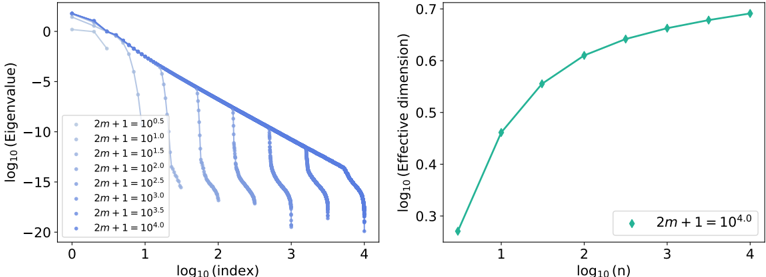
\n ## Charts: Eigenvalue Spectrum and Effective Dimension ### Overview The image presents two charts. The left chart displays the log10 of the Eigenvalues versus the log10 of the Index for different values of '2m+1'. The right chart shows the log10 of the Effective Dimension versus the log10 of 'n', also for a specific value of '2m+1'. ### Components/Axes **Left Chart:** * **X-axis:** log10(Index), ranging approximately from 0 to 4. * **Y-axis:** log10(Eigenvalue), ranging approximately from -20 to 0. * **Legend:** Located in the top-left corner. Contains the following labels: * 2m+1 = 10^5 (Blue) * 2m+1 = 10^4 (Blue) * 2m+1 = 10^3.5 (Blue) * 2m+1 = 10^3 (Blue) * 2m+1 = 10^2.5 (Blue) * 2m+1 = 10^2 (Blue) * 2m+1 = 10^1 (Blue) **Right Chart:** * **X-axis:** log10(n), ranging approximately from 0 to 4. * **Y-axis:** log10(Effective dimension), ranging approximately from 0.3 to 0.7. * **Legend:** Located in the bottom-right corner. Contains the following label: * 2m+1 = 10^4 (Teal) ### Detailed Analysis or Content Details **Left Chart:** * **2m+1 = 10^5:** The line starts at approximately log10(Eigenvalue) = -0.5 at log10(Index) = 0, and decreases steadily to approximately log10(Eigenvalue) = -19 at log10(Index) = 4. * **2m+1 = 10^4:** The line starts at approximately log10(Eigenvalue) = -1.5 at log10(Index) = 0, and decreases steadily to approximately log10(Eigenvalue) = -18 at log10(Index) = 4. * **2m+1 = 10^3.5:** The line starts at approximately log10(Eigenvalue) = -2.5 at log10(Index) = 0, and decreases steadily to approximately log10(Eigenvalue) = -17 at log10(Index) = 4. * **2m+1 = 10^3:** The line starts at approximately log10(Eigenvalue) = -3.5 at log10(Index) = 0, and decreases steadily to approximately log10(Eigenvalue) = -16 at log10(Index) = 4. * **2m+1 = 10^2.5:** The line starts at approximately log10(Eigenvalue) = -4.5 at log10(Index) = 0, and decreases steadily to approximately log10(Eigenvalue) = -15 at log10(Index) = 4. * **2m+1 = 10^2:** The line starts at approximately log10(Eigenvalue) = -5.5 at log10(Index) = 0, and decreases steadily to approximately log10(Eigenvalue) = -14 at log10(Index) = 4. * **2m+1 = 10^1:** The line starts at approximately log10(Eigenvalue) = -6.5 at log10(Index) = 0, and decreases steadily to approximately log10(Eigenvalue) = -13 at log10(Index) = 4. **Right Chart:** * **2m+1 = 10^4:** The line starts at approximately log10(Effective dimension) = 0.32 at log10(n) = 0, increases rapidly to approximately log10(Effective dimension) = 0.65 at log10(n) = 3, and plateaus to approximately log10(Effective dimension) = 0.68 at log10(n) = 4. ### Key Observations * In the left chart, all lines exhibit a similar downward trend, indicating that the Eigenvalues decrease as the Index increases. The lines are parallel, suggesting that the rate of decrease is consistent across different values of '2m+1'. Higher values of '2m+1' correspond to higher Eigenvalues for a given index. * In the right chart, the effective dimension increases with 'n' and appears to saturate at higher values of 'n'. ### Interpretation The left chart shows the eigenvalue spectrum, which is a measure of the variance explained by each principal component. The rapid decay of the eigenvalues suggests that the data is concentrated in a few dimensions. The different curves represent the eigenvalue spectrum for different values of '2m+1', which likely represents a parameter controlling the complexity or resolution of the system. The right chart shows how the effective dimension of the data changes as the size of the data ('n') increases. The initial rapid increase in effective dimension indicates that adding more data points initially reveals more independent directions of variation. The saturation at higher values of 'n' suggests that the data eventually becomes fully spanned by the available dimensions. The relationship between the two charts is that the effective dimension is related to the number of significant eigenvalues. As 'n' increases, more eigenvalues become significant, leading to a higher effective dimension. The value of '2m+1' influences the overall scale of the eigenvalues and the rate at which the effective dimension increases. The saturation of the effective dimension suggests that the data is ultimately limited by the intrinsic dimensionality of the underlying system.