## Line Graph with Spectrogram: Bivariate Probability Density and Temporal Signal Analysis
### Overview
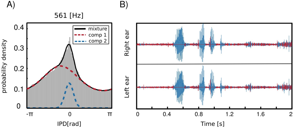
The image contains two panels:
- **Panel A**: A probability density distribution graph showing a mixture of two components (comp 1 and comp 2) at 561 Hz.
- **Panel B**: A spectrogram visualizing temporal signals for right and left ears, with red and blue color coding.
### Components/Axes
#### Panel A
- **X-axis**: IPD[rad] (Interaural Phase Difference in radians), labeled with markers:
- `-TT` (left boundary, approximate -π radians)
- `0` (center)
- `TT` (right boundary, approximate +π radians)
- **Y-axis**: Probability density (0 to 0.4).
- **Legend**:
- **Black solid line**: Mixture (combined signal of comp 1 and comp 2).
- **Red dashed line**: Component 1 (comp 1).
- **Blue dashed line**: Component 2 (comp 2).
#### Panel B
- **X-axis**: Time [s], ranging from 0 to 2 seconds, marked at 0.4s intervals.
- **Y-axis**: Ear labels:
- **Right ear** (top subplot).
- **Left ear** (bottom subplot).
- **Color coding**:
- **Red**: Likely corresponds to comp 1 (Panel A).
- **Blue**: Likely corresponds to comp 2 (Panel A).
### Detailed Analysis
#### Panel A
- The **mixture** (black solid line) peaks sharply at IPD = 0 rad, with a probability density of ~0.4.
- **Comp 1** (red dashed line) has a broader peak centered near 0 rad, with a maximum probability density of ~0.3.
- **Comp 2** (blue dashed line) has a narrower, lower peak at ~0 rad, with a maximum probability density of ~0.15.
- The distribution is symmetric around IPD = 0, suggesting balanced contributions from both components.
#### Panel B
- **Right ear**:
- Dominated by **blue spikes** (comp 2), with periodic bursts at ~0.4s, 0.8s, and 1.2s.
- Red spikes (comp 1) are less frequent and weaker.
- **Left ear**:
- Dominated by **red spikes** (comp 1), with similar temporal periodicity to the right ear.
- Blue spikes (comp 2) are sparse and weaker.
- Both ears show overlapping noise floors (gray shading), indicating background interference.
### Key Observations
1. **Component Dominance**:
- Comp 1 (red) dominates the left ear, while comp 2 (blue) dominates the right ear.
- The mixture (black) reflects a balanced combination of both components.
2. **Temporal Periodicity**:
- Spikes in both ears recur every ~0.4s, suggesting a 2.5 Hz fundamental frequency (561 Hz harmonics).
3. **Asymmetry**:
- The right ear exhibits stronger comp 2 activity, while the left ear shows stronger comp 1 activity.
### Interpretation
- **Signal Composition**:
The mixture in Panel A represents a bivariate probability distribution of interaural phase differences, with comp 1 and comp 2 contributing distinct spectral features. The sharper peak of the mixture at IPD = 0 suggests constructive interference between the components.
- **Ear-Specific Processing**:
The spectrogram (Panel B) reveals lateralized processing: the right ear emphasizes comp 2 (blue), while the left ear emphasizes comp 1 (red). This asymmetry may reflect directional hearing or neural filtering mechanisms.
- **Temporal Dynamics**:
The periodic spikes in both ears align with the 561 Hz frequency, indicating a sinusoidal or harmonic signal. The phase difference (IPD) distribution in Panel A likely governs the spatial localization of these temporal events.
- **Anomalies**:
The weaker blue spikes in the left ear and red spikes in the right ear suggest potential cross-talk or attenuation in interaural signal transmission.
### Technical Implications
This data demonstrates how bivariate probability distributions (Panel A) can model interaural phase differences, while spectrograms (Panel B) visualize the temporal-spatial dynamics of auditory signals. The asymmetry between ears highlights the role of binaural processing in sound localization and neural encoding.