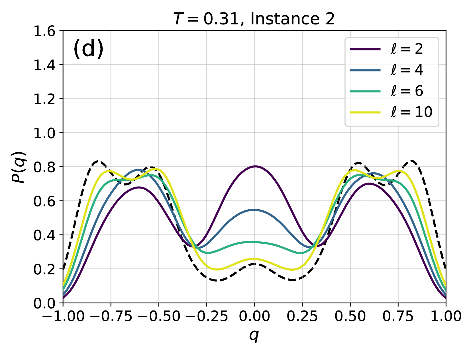
\n ## Line Chart: Probability Distribution P(q) for Different ℓ Values at T=0.31 ### Overview The image is a line chart (plot) labeled "(d)" in the top-left corner, with the title "T = 0.31, Instance 2" centered at the top. It displays the probability distribution function P(q) as a function of the variable q for four different values of a parameter ℓ, plus an additional dashed black reference curve. The chart is presented on a white background with a light gray grid. ### Components/Axes * **Title:** "T = 0.31, Instance 2" * **Panel Label:** "(d)" located in the top-left corner of the plot area. * **X-Axis:** * **Label:** "q" (centered below the axis). * **Scale:** Linear, ranging from -1.00 to 1.00. * **Major Ticks/Markers:** -1.00, -0.75, -0.50, -0.25, 0.00, 0.25, 0.50, 0.75, 1.00. * **Y-Axis:** * **Label:** "P(q)" (centered and rotated vertically to the left of the axis). * **Scale:** Linear, ranging from 0.0 to 1.6. * **Major Ticks/Markers:** 0.0, 0.2, 0.4, 0.6, 0.8, 1.0, 1.2, 1.4, 1.6. * **Legend:** * **Position:** Top-right corner of the plot area. * **Content:** Maps line colors to values of ℓ. * Dark Purple Line: ℓ = 2 * Blue Line: ℓ = 4 * Green Line: ℓ = 6 * Yellow Line: ℓ = 10 * **Note:** A dashed black line is also present in the plot but is not included in the legend. ### Detailed Analysis The chart plots five distinct curves. All curves are symmetric about q = 0.00. 1. **Dashed Black Line (Reference):** * **Trend:** Exhibits three sharp, distinct peaks. The central peak at q=0.00 is the lowest (~0.22). The two side peaks, located at approximately q = ±0.70, are the highest on the entire chart, reaching a P(q) value of ~0.83. Deep troughs occur at approximately q = ±0.25, with P(q) ~0.15. * **Key Points (Approximate):** * Peak 1: (q ≈ -0.70, P(q) ≈ 0.83) * Trough 1: (q ≈ -0.25, P(q) ≈ 0.15) * Central Peak: (q = 0.00, P(q) ≈ 0.22) * Trough 2: (q ≈ 0.25, P(q) ≈ 0.15) * Peak 2: (q ≈ 0.70, P(q) ≈ 0.83) 2. **Purple Line (ℓ = 2):** * **Trend:** Shows three broader, smoother peaks compared to the dashed line. The central peak at q=0.00 is the highest of all the colored lines, reaching P(q) ≈ 0.80. The side peaks, located near q = ±0.60, are lower, at P(q) ≈ 0.70. Troughs are at approximately q = ±0.30, with P(q) ≈ 0.35. * **Key Points (Approximate):** * Side Peak: (q ≈ -0.60, P(q) ≈ 0.70) * Trough: (q ≈ -0.30, P(q) ≈ 0.35) * Central Peak: (q = 0.00, P(q) ≈ 0.80) * Trough: (q ≈ 0.30, P(q) ≈ 0.35) * Side Peak: (q ≈ 0.60, P(q) ≈ 0.70) 3. **Blue Line (ℓ = 4):** * **Trend:** Also has three peaks. The central peak is significantly lower than that of ℓ=2, at P(q) ≈ 0.55. The side peaks, near q = ±0.55, are the highest for this curve, at P(q) ≈ 0.78. Troughs are at approximately q = ±0.25, with P(q) ≈ 0.32. * **Key Points (Approximate):** * Side Peak: (q ≈ -0.55, P(q) ≈ 0.78) * Trough: (q ≈ -0.25, P(q) ≈ 0.32) * Central Peak: (q = 0.00, P(q) ≈ 0.55) * Trough: (q ≈ 0.25, P(q) ≈ 0.32) * Side Peak: (q ≈ 0.55, P(q) ≈ 0.78) 4. **Green Line (ℓ = 6):** * **Trend:** Three peaks, with the central peak lower still. The central peak at q=0.00 is at P(q) ≈ 0.36. The side peaks, near q = ±0.50, are at P(q) ≈ 0.75. Troughs are at approximately q = ±0.20, with P(q) ≈ 0.30. * **Key Points (Approximate):** * Side Peak: (q ≈ -0.50, P(q) ≈ 0.75) * Trough: (q ≈ -0.20, P(q) ≈ 0.30) * Central Peak: (q = 0.00, P(q) ≈ 0.36) * Trough: (q ≈ 0.20, P(q) ≈ 0.30) * Side Peak: (q ≈ 0.50, P(q) ≈ 0.75) 5. **Yellow Line (ℓ = 10):** * **Trend:** Three peaks. The central peak is the lowest among all curves, at P(q) ≈ 0.25. The side peaks, near q = ±0.45, are at P(q) ≈ 0.79. Troughs are at approximately q = ±0.15, with P(q) ≈ 0.20. * **Key Points (Approximate):** * Side Peak: (q ≈ -0.45, P(q) ≈ 0.79) * Trough: (q ≈ -0.15, P(q) ≈ 0.20) * Central Peak: (q = 0.00, P(q) ≈ 0.25) * Trough: (q ≈ 0.15, P(q) ≈ 0.20) * Side Peak: (q ≈ 0.45, P(q) ≈ 0.79) ### Key Observations 1. **Symmetry:** All distributions are perfectly symmetric around q = 0.00. 2. **Central Peak Suppression:** As the parameter ℓ increases from 2 to 10, the height of the central peak at q=0.00 systematically decreases (from ~0.80 to ~0.25). 3. **Side Peak Consistency:** The height of the side peaks remains relatively stable across different ℓ values, clustering between P(q) ≈ 0.70 and 0.79. Their position shifts slightly inward (closer to q=0) as ℓ increases. 4. **Dashed Line Anomaly:** The dashed black line has the most pronounced side peaks and the deepest troughs, suggesting it may represent a theoretical limit, a different model, or a baseline case (e.g., ℓ → ∞ or a non-interacting system). 5. **Trough Depth:** The depth of the troughs between the central and side peaks generally decreases (becomes shallower) as ℓ increases. ### Interpretation This chart likely illustrates the probability distribution of an order parameter `q` in a statistical physics or machine learning context (e.g., spin glasses, neural networks, or optimization landscapes) at a fixed temperature T=0.31 for a specific system instance. * **Effect of ℓ:** The parameter ℓ appears to control the "localization" or "concentration" of probability. A smaller ℓ (e.g., 2) favors a high probability at the symmetric state (q=0). As ℓ increases, probability mass is redistributed from the center to the side peaks, indicating a transition towards states with non-zero `q` (possibly ordered or metastable states). The system becomes less likely to be found in the q=0 state. * **Multi-stability:** The presence of three distinct peaks for all ℓ values suggests the system has three metastable states or preferred configurations: one at q=0 and two symmetrically placed at ±q*. The relative stability of these states changes with ℓ. * **Dashed Line Significance:** The dashed line, with its extreme peaks and troughs, may represent the "ground truth" distribution, the result from a mean-field theory, or the distribution in the thermodynamic limit. The colored lines for finite ℓ show how the distribution deviates from this reference, with larger ℓ bringing the side peak positions closer to the dashed line's peaks but not matching their height or the depth of the troughs. * **Underlying Phenomenon:** The data demonstrates a classic symmetry-breaking scenario controlled by the parameter ℓ. The system's behavior evolves from being centered around the symmetric point (q=0) to favoring asymmetric, symmetry-broken states (q ≠ 0) as ℓ grows.