## Diagram: Monte Carlo Tree Search (MCTS) with Potential Progressive Widening
### Overview
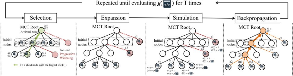
The image is a technical diagram illustrating the four sequential stages of the Monte Carlo Tree Search (MCTS) algorithm, augmented with a concept called "Potential Progressive Widening." The process is depicted as a cyclical flow, repeated for a specified number of iterations (T). The diagram uses tree structures to visualize the state of the search tree at each stage.
### Components/Axes
The diagram is segmented into four primary stages, arranged horizontally from left to right, each contained within a dashed vertical boundary:
1. **Selection**
2. **Expansion**
3. **Simulation**
4. **Backpropagation**
A large, black, curved arrow at the top connects the end of the "Backpropagation" stage back to the beginning of the "Selection" stage, labeled with the text: **"Repeated until evaluating g(·) for T times"**.
**Legend (Bottom Left):**
* A green arrow is labeled: **"To a child node with the largest UCT(·)"**.
* A red dashed circle is labeled: **"Potential Progressive Widening"**.
**Common Elements in Each Stage:**
* **MCT Root:** A central white circle at the top of each tree, labeled **"MCT Root"**. In the first stage, it is further annotated as **"A virtual node"**.
* **Initial nodes:** A set of nodes directly connected to the root, enclosed in a gray dotted rectangle and labeled **"Initial nodes"**.
* **Node Annotations:** Nodes contain mathematical symbols and icons. Common annotations include:
* `N(·)`: Visit count.
* `Q(·)`: Action value.
* `U(·)`: Exploration bonus term (part of the UCT formula).
* Icons: Small square icons depicting what appears to be a document or state symbol.
* **Child Node Labels:** In later stages, child nodes are given specific labels like `e1`, `e2`, `c2`, `m1`, `w1`, `s1`.
### Detailed Analysis
**1. Selection Stage:**
* The MCT Root is shown with a green arrow pointing from it to one of its child nodes within the "Initial nodes" group.
* This child node is further annotated with `N(·)`, `Q(·)`, and `U(·)`.
* A red dashed circle labeled **"Potential Progressive Widening"** is positioned to the right of the initial nodes, indicating a decision point for adding new nodes.
**2. Expansion Stage:**
* The tree has grown. New child nodes (labeled `e1`, `e2`) have been added to the "Initial nodes."
* The node `e2` is highlighted with a red dashed circle, indicating it is the subject of the "Potential Progressive Widening" action in this step.
* The tree now shows a second level of children below the initial nodes.
**3. Simulation Stage:**
* The tree is more developed. The node `e2` now has its own children (`c2`, `m1`, `w1`, `s1`).
* These leaf nodes are annotated with specific values, for example:
* Node `c2`: `N(·)=1`, `Q(·)=g(·)`.
* Node `m1`: `N(·)=1`, `Q(·)=g(·)`.
* The red dashed circle for "Potential Progressive Widening" is now around node `e1`.
**4. Backpropagation Stage:**
* The path from a leaf node back to the root is highlighted in orange.
* The highlighted path goes: a leaf node (e.g., `s1`) -> its parent (`e2`) -> the MCT Root.
* The nodes along this path (`e2` and the MCT Root) are filled with an orange color.
* Annotations on the orange nodes show updated values. For example, the MCT Root now shows `N(·)=1` and `Q(·)=g(·)`.
* The red dashed circle for "Potential Progressive Widening" is now around the MCT Root itself.
### Key Observations
1. **Iterative Process:** The diagram clearly shows MCTS as a loop, not a one-pass algorithm. The state of the tree evolves with each cycle.
2. **Tree Growth:** The tree visibly grows in complexity from the Selection to the Simulation stage, adding new nodes and levels.
3. **Value Propagation:** The Backpropagation stage visually demonstrates how the result of a simulation (the value `g(·)`) is propagated back up the tree, updating the statistics (`N` and `Q`) of ancestor nodes.
4. **Progressive Widening Integration:** The "Potential Progressive Widening" element (red dashed circle) moves to different nodes in each stage, suggesting it is a dynamic process applied to specific nodes during the search to manage branching factor.
5. **UCT Guidance:** The green arrow in the Selection stage explicitly shows that the UCT (Upper Confidence bound for Trees) formula is used to select which node to explore.
### Interpretation
This diagram is a pedagogical tool explaining an enhanced version of the MCTS algorithm. The core MCTS cycle (Selection -> Expansion -> Simulation -> Backpropagation) is standard. The key addition is the **"Potential Progressive Widening"** mechanism.
* **What it suggests:** In standard MCTS, all possible actions from a state might be considered. Progressive Widening is a technique used in large or continuous action spaces. Instead of expanding all children at once, the algorithm selectively adds new action nodes ("widens" the tree) only when a node has been visited a certain number of times. The diagram shows this widening being applied to different nodes (`e2`, `e1`, then the Root) at different stages, implying it's a conditional operation.
* **How elements relate:** The Selection phase uses UCT to balance exploration and exploitation. The Expansion phase, guided by Progressive Widening, adds new nodes to the tree. The Simulation (or Rollout) phase estimates the value of a new node. The Backpropagation phase updates the tree's statistics with this new information. The loop repeats, allowing the algorithm to focus computation on promising regions of the search space.
* **Notable aspects:** The use of a "virtual" root node and the specific labeling of child nodes (`e1`, `e2`, `c2`, etc.) suggest this diagram might be from a paper or context where these labels correspond to specific actions or states in a problem domain (e.g., game moves, robotic decisions). The notation `g(·)` represents the outcome or reward function being evaluated. The diagram effectively communicates how an intelligent search process can iteratively build and refine a decision tree under computational constraints.