# Technical Data Extraction: WSe2 Current Density and Flow Maps
This document provides a detailed technical extraction of the data contained in the provided image, which consists of two side-by-side scientific plots (labeled 'g' and 'h') representing physical simulations of Tungsten Diselenide ($WSe_2$).
## 1. General Metadata
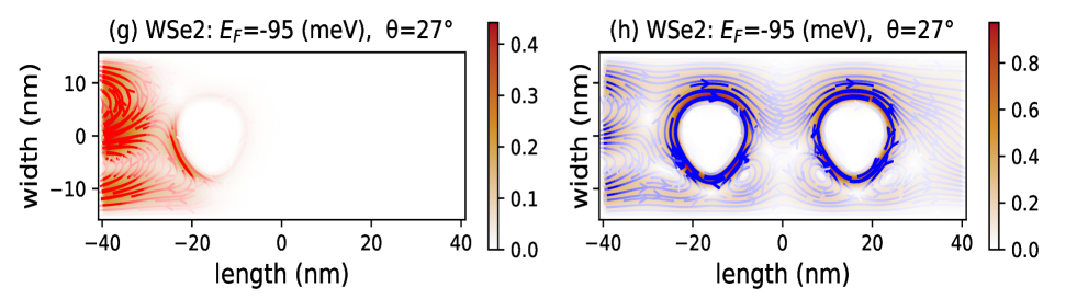
* **Material:** $WSe_2$ (Tungsten Diselenide)
* **Fermi Energy ($E_F$):** -95 meV
* **Angle ($\theta$):** 27°
* **Primary Language:** English
---
## 2. Component Isolation: Plot (g)
### Header & Labels
* **Title:** (g) $WSe_2$: $E_F$=-95 (meV), $\theta$=27°
* **Y-axis Label:** width (nm)
* **X-axis Label:** length (nm)
### Axis Scales
* **X-axis Range:** -40 to 40 nm (Markers at -40, -20, 0, 20, 40)
* **Y-axis Range:** -10 to 10 nm (Markers at -10, 0, 10)
### Colorbar (Legend)
* **Location:** Right side of plot (g)
* **Scale:** 0.0 to 0.4 (Linear gradient from white/light orange to dark red)
* **Function:** Represents magnitude (likely current density or local density of states).
### Data Content & Trends
* **Visual Trend:** The data is concentrated on the left side of the plot (negative length). The right side (length > -10 nm) is largely empty/white, indicating zero or near-zero values.
* **Flow Features:**
* There is a high-intensity region (dark red, ~0.4 on the scale) between length -40 and -25 nm.
* Streamlines (red lines) show a turbulent or circulating flow pattern on the far left.
* A distinct "void" or circular exclusion zone is visible centered approximately at length = -15 nm, width = 0 nm.
* A high-intensity "boundary" (dark red) wraps around the left edge of this void.
---
## 3. Component Isolation: Plot (h)
### Header & Labels
* **Title:** (h) $WSe_2$: $E_F$=-95 (meV), $\theta$=27°
* **Y-axis Label:** width (nm)
* **X-axis Label:** length (nm)
### Axis Scales
* **X-axis Range:** -40 to 40 nm (Markers at -40, -20, 0, 20, 40)
* **Y-axis Range:** -10 to 10 nm (Markers at -10, 0, 10)
### Colorbar (Legend)
* **Location:** Right side of plot (h)
* **Scale:** 0.0 to 0.8 (Linear gradient from white/light orange to dark red)
* **Note:** The scale in (h) is double the magnitude of the scale in (g).
### Data Content & Trends
* **Visual Trend:** Unlike plot (g), the data in (h) spans the entire length of the channel (-40 to 40 nm).
* **Flow Features:**
* **Vortex Structures:** There are two prominent circular "voids" or obstacles centered at approximately **length = -18 nm** and **length = +18 nm**.
* **Circulation:** Blue streamlines with arrows indicate a strong clockwise circulation around these two centers.
* **Intensity:** The highest intensity (dark red, ~0.8) occurs at the immediate boundaries of these circular structures.
* **Background Flow:** Between the vortices and at the far left/right edges, the flow appears more laminar but contains smaller secondary eddies.
* **Symmetry:** The plot shows a high degree of periodicity or symmetry relative to the length = 0 axis.
---
## 4. Comparative Analysis
| Feature | Plot (g) | Plot (h) |
| :--- | :--- | :--- |
| **Max Magnitude** | 0.4 | 0.8 |
| **Spatial Coverage** | Left-heavy (localized) | Full channel (distributed) |
| **Primary Features** | Single partial vortex/boundary | Two complete counter-circulating vortices |
| **Streamline Color** | Red | Blue (with directional arrows) |
**Summary:** These plots likely represent different components of a current or wave function (e.g., longitudinal vs. transverse or different valley contributions) for $WSe_2$ under specific energy and angular conditions. Plot (h) shows a much more developed and higher-magnitude flow pattern compared to the localized behavior in plot (g).