## Diagram: Transformation of a Sparse Grid to a Dense Matrix
### Overview
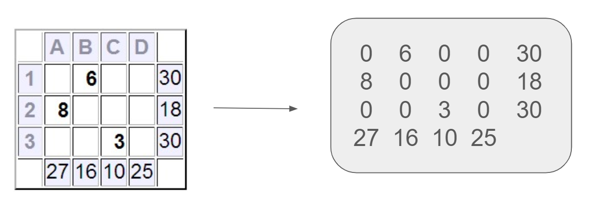
The image displays a two-part diagram illustrating the transformation of a sparse, labeled grid (left) into a dense numerical matrix (right). An arrow points from the left grid to the right matrix, indicating a direct mapping or conversion process. This diagram is characteristic of representations used in operations research, specifically for formulating transportation or assignment problems.
### Components/Axes
**Left Component: Sparse Grid with Totals**
* **Structure:** A 3-row by 4-column grid.
* **Row Labels (Vertical Axis):** `1`, `2`, `3` (positioned to the left of each row).
* **Column Labels (Horizontal Axis):** `A`, `B`, `C`, `D` (positioned above each column).
* **Filled Cells (Data Points):**
* Cell at intersection of Row `1`, Column `B`: `6`
* Cell at intersection of Row `2`, Column `A`: `8`
* Cell at intersection of Row `3`, Column `C`: `3`
* **Row Totals (Right of Grid):** A column of numbers aligned with each row.
* Row `1` total: `30`
* Row `2` total: `18`
* Row `3` total: `30`
* **Column Totals (Below Grid):** A row of numbers aligned with each column.
* Column `A` total: `27`
* Column `B` total: `16`
* Column `C` total: `10`
* Column `D` total: `25`
**Right Component: Dense Matrix**
* **Structure:** A 4-row by 5-column matrix contained within a rounded rectangle.
* **Content (Row-wise):**
* **Row 1:** `0`, `6`, `0`, `0`, `30`
* **Row 2:** `8`, `0`, `0`, `0`, `18`
* **Row 3:** `0`, `0`, `3`, `0`, `30`
* **Row 4:** `27`, `16`, `10`, `25` (Note: This row contains only four values, aligned under the first four columns).
**Connector:** A simple right-pointing arrow (`→`) links the two components, indicating the direction of transformation.
### Detailed Analysis
The transformation maps the sparse grid and its marginal totals into a single, consolidated matrix.
1. **Mapping of Grid Values:** The non-zero values from the 3x4 grid (`6`, `8`, `3`) are placed into the first three rows and first four columns of the dense matrix at their corresponding (row, column) positions. All other cells in this 3x4 sub-matrix are filled with `0`.
2. **Incorporation of Row Totals:** The row totals (`30`, `18`, `30`) from the left are placed as the fifth element in the first three rows of the dense matrix.
3. **Incorporation of Column Totals:** The column totals (`27`, `16`, `10`, `25`) from the left are placed as the fourth row of the dense matrix, occupying the first four columns. The fifth column of this fourth row is empty/absent in the visual representation.
4. **Data Consistency Check:** The sum of the row totals (30 + 18 + 30 = 78) equals the sum of the column totals (27 + 16 + 10 + 25 = 78), indicating a balanced system, which is a fundamental requirement for a feasible solution in a transportation problem.
### Key Observations
* **Sparsity to Density:** The left grid is sparse (only 3 of 12 cells filled), while the right matrix is dense, with zeros explicitly shown.
* **Structural Transformation:** The diagram converts a "tableau" view with separate marginal totals into a unified matrix format where totals are integrated as an additional row and column.
* **Visual Anomaly:** The fourth row of the dense matrix has only four entries, breaking the rectangular pattern. This visually emphasizes that the column totals correspond only to the original four columns (A-D).
### Interpretation
This diagram almost certainly illustrates the **initial setup for a Transportation Problem** in linear programming or operations research.
* **Left Grid:** Represents the **cost matrix** or **initial allocation matrix**. The numbers `6`, `8`, `3` likely represent the cost per unit to ship from a source (rows 1,2,3) to a destination (columns A,B,C,D), or possibly an initial feasible allocation of units. The row totals (`30`, `18`, `30`) represent the **supply** at each source, and the column totals (`27`, `16`, `10`, `25`) represent the **demand** at each destination.
* **Right Matrix:** Represents the **standard tableau form** used in the Transportation Simplex Method (or similar algorithms). In this tableau:
* The top-left 3x4 block holds the unit costs or allocations.
* The fifth column holds the supply values.
* The fourth row holds the demand values.
* The bottom-right cell (implied but not shown) would typically hold the total cost or serve as a pivot point.
* **Purpose of Transformation:** Converting the problem into this dense matrix format allows for systematic application of algorithms (like the Northwest Corner Rule, Least Cost Method, or Vogel's Approximation Method) to find an initial basic feasible solution, which is then optimized. The zeros represent non-basic variables (routes not used in the initial solution).
The diagram serves as a clear visual guide for how to structure problem data from a descriptive format into a computational format ready for algorithmic solving.