## Chart/Diagram Type: Multi-Panel Plot
### Overview
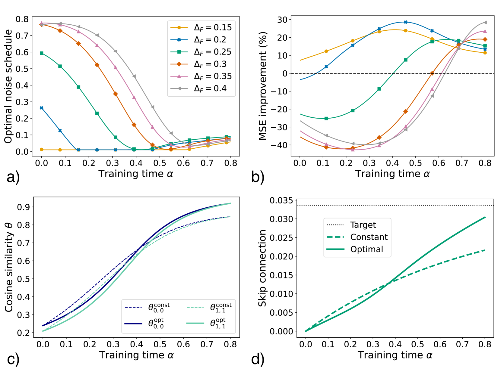
The image presents four plots (a, b, c, d) that analyze the effects of different noise schedules on a machine learning model during training. The plots explore optimal noise schedules, MSE improvement, cosine similarity, and skip connections as functions of training time.
### Components/Axes
**Panel a: Optimal Noise Schedule**
* **Title:** Optimal noise schedule
* **X-axis:** Training time α, ranging from 0.0 to 0.8 in increments of 0.1.
* **Y-axis:** Optimal noise schedule, ranging from 0.0 to 0.8 in increments of 0.1.
* **Legend (Top-Right):**
* Yellow: ΔF = 0.15
* Blue: ΔF = 0.2
* Green: ΔF = 0.25
* Orange: ΔF = 0.3
* Pink: ΔF = 0.35
* Gray: ΔF = 0.4
**Panel b: MSE Improvement**
* **Title:** MSE improvement (%)
* **X-axis:** Training time α, ranging from 0.0 to 0.8 in increments of 0.1.
* **Y-axis:** MSE improvement (%), ranging from -40 to 30 in increments of 10.
* **Horizontal dashed line:** at y = 0
* **Legend:** (Refer to Panel a for color correspondence to ΔF values)
* Yellow: ΔF = 0.15
* Blue: ΔF = 0.2
* Green: ΔF = 0.25
* Orange: ΔF = 0.3
* Pink: ΔF = 0.35
* Gray: ΔF = 0.4
**Panel c: Cosine Similarity**
* **Title:** Cosine similarity θ
* **X-axis:** Training time α, ranging from 0.0 to 0.8 in increments of 0.1.
* **Y-axis:** Cosine similarity θ, ranging from 0.2 to 0.9 in increments of 0.1.
* **Legend (Center-Right):**
* Dashed Dark Blue: θ<sup>const</sup><sub>0,0</sub>
* Solid Dark Blue: θ<sup>opt</sup><sub>0,0</sub>
* Dashed Light Green: θ<sup>const</sup><sub>1,1</sub>
* Solid Light Green: θ<sup>opt</sup><sub>1,1</sub>
**Panel d: Skip Connection**
* **Title:** Skip connection
* **X-axis:** Training time α, ranging from 0.0 to 0.8 in increments of 0.1.
* **Y-axis:** Skip connection, ranging from 0.000 to 0.035 in increments of 0.005.
* **Legend (Right):**
* Dotted Black: Target
* Dashed Green: Constant
* Solid Green: Optimal
### Detailed Analysis
**Panel a: Optimal Noise Schedule**
* **ΔF = 0.15 (Yellow):** Remains relatively constant at approximately 0.02 across all training times.
* **ΔF = 0.2 (Blue):** Starts at approximately 0.25 and decreases sharply to approximately 0.02 by α = 0.2, then remains constant.
* **ΔF = 0.25 (Green):** Starts at approximately 0.6 and decreases to approximately 0.07 by α = 0.5, then remains constant.
* **ΔF = 0.3 (Orange):** Starts at approximately 0.75 and decreases to approximately 0.07 by α = 0.6, then remains constant.
* **ΔF = 0.35 (Pink):** Starts at approximately 0.78 and decreases to approximately 0.08 by α = 0.7, then remains constant.
* **ΔF = 0.4 (Gray):** Starts at approximately 0.78 and decreases to approximately 0.08 by α = 0.7, then remains constant.
**Panel b: MSE Improvement**
* **ΔF = 0.15 (Yellow):** Increases from approximately 8% to 22% as α increases from 0.0 to 0.8.
* **ΔF = 0.2 (Blue):** Increases from approximately -2% to 20% as α increases from 0.0 to 0.8, peaking at α = 0.4 with a value of 25%.
* **ΔF = 0.25 (Green):** Decreases from approximately -25% to -18% until α = 0.4, then increases to approximately 15% at α = 0.8.
* **ΔF = 0.3 (Orange):** Decreases from approximately -35% to -40% until α = 0.2, then increases to approximately 20% at α = 0.8.
* **ΔF = 0.35 (Pink):** Decreases from approximately -35% to -42% until α = 0.2, then increases to approximately 22% at α = 0.8.
* **ΔF = 0.4 (Gray):** Decreases from approximately -28% to -42% until α = 0.2, then increases to approximately 30% at α = 0.8.
**Panel c: Cosine Similarity**
* **θ<sup>const</sup><sub>0,0</sub> (Dashed Dark Blue):** Increases from approximately 0.23 to 0.83 as α increases from 0.0 to 0.8.
* **θ<sup>opt</sup><sub>0,0</sub> (Solid Dark Blue):** Increases from approximately 0.23 to 0.92 as α increases from 0.0 to 0.8.
* **θ<sup>const</sup><sub>1,1</sub> (Dashed Light Green):** Increases from approximately 0.23 to 0.85 as α increases from 0.0 to 0.8.
* **θ<sup>opt</sup><sub>1,1</sub> (Solid Light Green):** Increases from approximately 0.23 to 0.92 as α increases from 0.0 to 0.8.
**Panel d: Skip Connection**
* **Target (Dotted Black):** Constant at approximately 0.034.
* **Constant (Dashed Green):** Increases linearly from approximately 0.00 to 0.022 as α increases from 0.0 to 0.8.
* **Optimal (Solid Green):** Increases from approximately 0.00 to 0.030 as α increases from 0.0 to 0.8.
### Key Observations
* **Optimal Noise Schedule (Panel a):** Higher ΔF values require a more aggressive reduction in noise early in training.
* **MSE Improvement (Panel b):** Higher ΔF values initially lead to worse MSE improvement, but eventually surpass lower ΔF values at later training times.
* **Cosine Similarity (Panel c):** Optimal noise schedules result in higher cosine similarity compared to constant noise schedules.
* **Skip Connection (Panel d):** Optimal skip connections approach the target value more closely than constant skip connections.
### Interpretation
The plots demonstrate the impact of varying noise schedules (ΔF) on model training. The results suggest that a carefully tuned noise schedule can significantly improve model performance, as measured by MSE improvement, cosine similarity, and skip connection values. Specifically, higher ΔF values, which represent more aggressive noise reduction, initially hinder performance but ultimately lead to better results at later stages of training. The cosine similarity plot indicates that optimal noise schedules help the model converge to a more desirable state. The skip connection plot shows that the optimal schedule allows the model to approach the target skip connection value more closely than a constant schedule.