\n
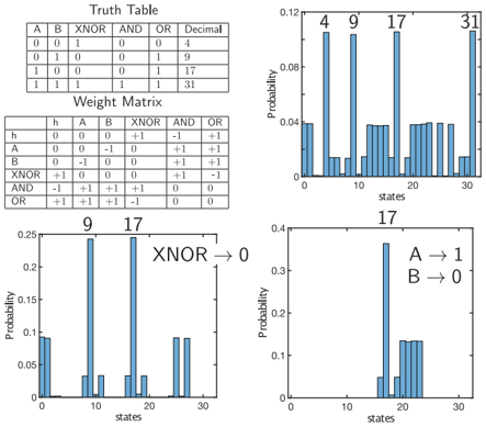
## Charts/Diagrams: Boolean Function Analysis & State Probabilities
### Overview
The image presents an analysis of Boolean functions (XNOR, AND, OR) using a truth table, a weight matrix, and probability distributions of states. The distributions appear to represent the probabilities of different states arising from the functions. There are four charts in total: a truth table, a weight matrix, and three histograms representing probability distributions.
### Components/Axes
* **Truth Table:** Columns labeled 'A', 'B', 'XNOR', 'AND', 'OR', 'Decimal'. Rows represent the input combinations (0,0), (0,1), (1,0), (1,1).
* **Weight Matrix:** Rows and columns labeled 'h', 'A', 'B', 'XNOR', 'AND', 'OR'. Values within the matrix are +1 or -1.
* **Histogram 1 (Top-Right):** X-axis labeled 'states', Y-axis labeled 'Probability'. The x-axis ranges from approximately 0 to 32. The histogram has peaks labeled '4', '9', '17', and '31'.
* **Histogram 2 (Bottom-Left):** X-axis labeled 'states', Y-axis labeled 'Probability'. The x-axis ranges from approximately 0 to 32. Peaks are labeled '9' and '17'. Text annotation: "XNOR → 0".
* **Histogram 3 (Bottom-Right):** X-axis labeled 'states', Y-axis labeled 'Probability'. The x-axis ranges from approximately 0 to 32. Peak is labeled '17'. Text annotation: "A → 1", "B → 0".
### Detailed Analysis or Content Details
**Truth Table:**
| A | B | XNOR | AND | OR | Decimal |
|---|---|---|---|---|---|
| 0 | 0 | 1 | 0 | 0 | 1 |
| 0 | 1 | 0 | 0 | 1 | 2 |
| 1 | 0 | 0 | 0 | 1 | 2 |
| 1 | 1 | 1 | 1 | 1 | 3 |
**Weight Matrix:**
| h | A | B | XNOR | AND | OR |
|---|---|---|---|---|---|
| h | 0 | 0 | 0 | +1 | -1 | +1 |
| A | 0 | 0 | +1 | 0 | -1 | -1 |
| B | 0 | +1 | 0 | 0 | -1 | -1 |
| XNOR | +1 | 0 | 0 | -1 | 0 | -1 |
| AND | +1 | 0 | -1 | 0 | 0 | 0 |
| OR | -1 | +1 | -1 | 0 | 0 | 0 |
**Histogram 1 (Top-Right):**
The histogram shows a distribution of probabilities across states. The highest probability is approximately 0.11 at state 9 and 17. There are smaller peaks at states 4 and 31, with probabilities around 0.09. The probability generally decreases between peaks.
* State 4: ~0.09
* State 9: ~0.11
* State 17: ~0.11
* State 31: ~0.09
**Histogram 2 (Bottom-Left):**
This histogram shows a bimodal distribution with peaks at states 9 and 17. The probability at state 9 is significantly higher, approximately 0.24. The probability at state 17 is approximately 0.16.
* State 9: ~0.24
* State 17: ~0.16
**Histogram 3 (Bottom-Right):**
This histogram shows a unimodal distribution with a strong peak at state 17. The probability at state 17 is approximately 0.35.
* State 17: ~0.35
### Key Observations
* The truth table defines the behavior of the XNOR, AND, and OR functions for all possible input combinations.
* The weight matrix appears to represent the weights associated with each variable and function in a neural network or similar model.
* The histograms show the probability distributions of states resulting from the Boolean functions.
* Histogram 2 (XNOR → 0) has peaks at states 9 and 17, suggesting these states are more likely when the XNOR function outputs 0.
* Histogram 3 (A → 1, B → 0) has a strong peak at state 17, indicating this state is highly probable when A is 1 and B is 0.
* The first histogram shows a more even distribution of probabilities across multiple states.
### Interpretation
The image demonstrates a connection between Boolean logic, weighted representations, and probabilistic state distributions. The truth table and weight matrix define the underlying logic, while the histograms visualize the resulting probabilities of different states. The annotations on the bottom histograms suggest a specific scenario where the XNOR function is forced to output 0, and another where A is 1 and B is 0. The differing distributions in each histogram indicate that the output probabilities are highly dependent on the input conditions and the underlying Boolean function. The weight matrix could be used to implement these functions in a neural network, and the histograms represent the network's output distribution. The data suggests that the XNOR function, when constrained to output 0, leads to a distribution favoring states 9 and 17, while the condition A=1, B=0 strongly favors state 17. The first histogram shows a more uniform distribution, indicating a less constrained or more complex scenario.