## Diagram: Meta-Learning Process
### Overview
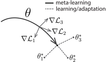
The image illustrates a meta-learning process, showing the trajectory of meta-learning and the adaptation steps towards task-specific optimal parameters. It depicts how meta-learning guides the model towards a parameter space that allows for efficient adaptation to new tasks.
### Components/Axes
* **θ (Theta)**: Represents the meta-learned parameters. It is shown as a curved solid black line, indicating the trajectory of meta-learning.
* **∇L1, ∇L2, ∇L3**: Gradients of the loss functions for different tasks. These are represented by gray arrows pointing towards the meta-learning trajectory.
* **θ\*1, θ\*2, θ\*3**: Task-specific optimal parameters after adaptation. These are represented by gray dots connected to the meta-learning trajectory by dashed gray lines.
* **Legend (Top-Right)**:
* Solid Black Line: "meta-learning"
* Dashed Gray Line: "learning/adaptation"
### Detailed Analysis
* The solid black line representing "meta-learning" shows a curved path, indicating the optimization process of the meta-learner.
* The gray arrows (∇L1, ∇L2, ∇L3) represent the gradients of the loss functions for different tasks. They point towards the meta-learning trajectory, suggesting that the meta-learner is being guided by these gradients.
* The dashed gray lines represent the adaptation process from the meta-learned parameters (θ) to the task-specific optimal parameters (θ\*1, θ\*2, θ\*3).
* The task-specific optimal parameters (θ\*1, θ\*2, θ\*3) are scattered around the end of the meta-learning trajectory, indicating that the meta-learner has found a parameter space that allows for efficient adaptation to different tasks.
### Key Observations
* The meta-learning trajectory (solid black line) is influenced by the gradients of the loss functions for different tasks (gray arrows).
* The adaptation process (dashed gray lines) leads to task-specific optimal parameters (gray dots).
* The meta-learning process aims to find a parameter space that allows for efficient adaptation to new tasks.
### Interpretation
The diagram illustrates the core concept of meta-learning, where a model learns how to learn. The meta-learner optimizes its parameters (θ) based on the gradients of the loss functions for different tasks (∇L1, ∇L2, ∇L3). This optimization process guides the meta-learner towards a parameter space that allows for efficient adaptation to new tasks, resulting in task-specific optimal parameters (θ\*1, θ\*2, θ\*3). The diagram effectively demonstrates how meta-learning enables a model to quickly adapt to new tasks with minimal training data.