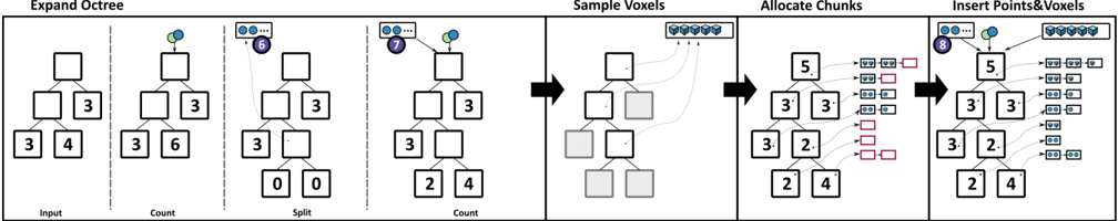
\n ## Diagram: Octree Expansion and Voxel Processing Pipeline ### Overview The image is a technical diagram illustrating a four-stage pipeline for processing spatial data using an octree structure. The pipeline progresses from left to right, showing how an initial octree is expanded, how voxels are sampled from it, how memory chunks are allocated, and finally how points and voxels are inserted into the structure. The diagram uses simplified tree representations with numbered nodes and visual metaphors for voxels and memory allocation. ### Components/Axes The diagram is segmented into four primary vertical sections, each with a title at the top: 1. **Expand Octree** (Leftmost section) 2. **Sample Voxels** (Center-left) 3. **Allocate Chunks** (Center-right) 4. **Insert Points & Voxels** (Rightmost section) Within the "Expand Octree" section, there are four sub-steps separated by vertical dashed lines, labeled at the bottom: * **Input** * **Count** * **Split** * **Count** (a second counting step) **Visual Components:** * **Tree Structures:** Represented by squares (nodes) connected by lines. Numbers inside the squares indicate a count or value associated with that node. * **Voxels:** Represented by small, light-blue cubes. A cluster of these cubes appears in a box in the "Sample Voxels" and "Insert Points & Voxels" stages. * **Points:** Represented by small, dark blue circles. They appear attached to specific tree nodes in the "Expand Octree" and "Insert Points & Voxels" stages. * **Chunks/Memory Blocks:** Represented by small, colored rectangles (pink and light blue outlines) in the "Allocate Chunks" and "Insert Points & Voxels" stages. * **Arrows:** Black arrows indicate the flow of the process between the four main stages. Faint gray lines in "Sample Voxels" show the sampling relationship. ### Detailed Analysis **1. Expand Octree Stage:** This stage shows the iterative process of refining an octree node. * **Input:** A simple tree with a root node and three child nodes. The children have the values `3`, `3`, and `4`. * **Count:** A point (dark blue circle) is associated with the root node. The child node values are updated to `3`, `3`, and `6`. * **Split:** The root node is split. It now has four child nodes. The original three children are retained, and a new, fourth child is added with a value of `0`. The point remains associated with the (now internal) root node. * **Count (Second):** After the split, the point is still at the root. The child node values are updated to `3`, `2`, `0`, and `4`. The node that previously had `6` now has `2` and `4`, indicating its data was distributed to its new children. **2. Sample Voxels Stage:** This stage is more abstract. It shows a tree structure (similar to the final tree from the previous stage) on the left. To its right is a box containing a 2x4 grid of light-blue voxel cubes. Faint gray lines connect specific nodes in the tree to this grid, suggesting that voxels are being sampled or associated with those nodes. **3. Allocate Chunks Stage:** This stage shows a tree with the following node values from top to bottom, left to right: `5` (root), `3`, `3`, `2`, `2`, `4`. To the right of the tree, there are columns of small, colored rectangles (pink and light blue outlines). These likely represent allocated memory chunks. The number of chunks appears to correspond to the node values (e.g., the root node `5` has a column of 5 chunks next to it). **4. Insert Points & Voxels Stage:** This is the final, composite stage. It combines elements from all previous stages: * The final tree structure from "Allocate Chunks" (nodes: `5`, `3`, `3`, `2`, `2`, `4`). * The cluster of light-blue voxel cubes from "Sample Voxels" is shown in a box at the top right. * The dark blue point is shown attached to the root node (`5`). * The columns of colored memory chunks from "Allocate Chunks" are shown to the right of their respective tree nodes. ### Key Observations * **Process Flow:** The diagram clearly depicts a sequential pipeline: Expand -> Sample -> Allocate -> Insert. * **Data Transformation:** The "Expand Octree" stage demonstrates how a node's data (value `6`) is redistributed to new child nodes (`2` and `4`) after a split operation. * **Visual Metaphors:** The diagram uses consistent visual metaphors: cubes for voxels, circles for points, and colored rectangles for memory chunks. * **Spatial Grounding:** The legend/labels are primarily in the top titles and bottom sub-step labels. The color coding is consistent: dark blue for points, light blue for voxels, pink/light blue outlines for chunks. The placement of the voxel box and chunk columns is consistently to the right of their associated tree structures. ### Interpretation This diagram illustrates a core algorithm in computer graphics, simulation, or spatial computing for dynamically managing a sparse 3D dataset. The octree is used to adaptively subdivide space only where data exists. * **What it demonstrates:** The pipeline shows how to efficiently handle a growing dataset. First, the octree structure is refined ("Expand") to accommodate new data at a finer resolution. Then, the actual volumetric data ("Voxels") is sampled from this structure. Next, memory ("Chunks") is allocated in a structured way that likely corresponds to the octree nodes for efficient access. Finally, new data points and voxels are inserted into this pre-allocated, organized structure. * **Relationships:** Each stage depends on the output of the previous one. The tree structure from the expansion stage defines where voxels are sampled. The final tree structure and node values determine the memory allocation pattern. The insertion stage populates this prepared structure. * **Notable Pattern:** The transition from the first "Count" (value `6`) to the post-split "Count" (values `2` and `4`) is a key detail. It shows the octree's purpose: breaking down a large, dense region (requiring a count of 6) into smaller, more manageable sub-regions (counts of 2 and 4) after spatial subdivision. This is fundamental to achieving efficient spatial queries and rendering.