\n
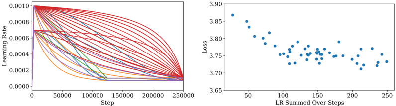
## Charts: Learning Rate Schedule and Loss vs. LR Summed Over Steps
### Overview
The image presents two charts side-by-side. The left chart depicts a learning rate schedule over training steps, showing multiple lines representing different learning rate trajectories. The right chart shows the loss function value plotted against the sum of learning rates over steps.
### Components/Axes
**Left Chart:**
* **X-axis:** "Step" ranging from 0 to 250000.
* **Y-axis:** "Learning Rate" ranging from 0.0000 to 0.00010.
* **Data Series:** Multiple lines, each representing a different learning rate schedule. No explicit labels are provided for each line.
**Right Chart:**
* **X-axis:** "LR Summed Over Steps" ranging from approximately 50 to 250.
* **Y-axis:** "Loss" ranging from approximately 3.65 to 3.90.
* **Data Series:** A scatter plot of individual data points.
### Detailed Analysis or Content Details
**Left Chart:**
The chart shows a collection of learning rate decay curves. All curves start at a relatively high learning rate (approximately 0.00009) at Step 0 and decrease over time. The decay is initially rapid, then slows down as the step number increases.
* The first ~50,000 steps show a steep decline in learning rate for all lines.
* Between 50,000 and 150,000 steps, the rate of decline slows significantly.
* After 150,000 steps, the learning rate plateaus, with most lines converging to a very low learning rate (approximately 0.00001).
* There is significant variation in the decay rates and final learning rates among the different lines.
**Right Chart:**
The chart displays a scatter plot showing the relationship between the sum of learning rates over steps and the corresponding loss value.
* The trend is generally downward, indicating that as the sum of learning rates increases, the loss decreases.
* The initial points (LR Summed Over Steps ~50) have a loss of approximately 3.85.
* Around LR Summed Over Steps ~150, the loss reaches a minimum of approximately 3.72.
* After LR Summed Over Steps ~150, the loss fluctuates around 3.75, with some points reaching as low as 3.70 and as high as 3.78.
* The points appear somewhat scattered, suggesting a noisy relationship between the sum of learning rates and the loss.
### Key Observations
* The learning rate schedule exhibits a decaying behavior, which is common in training deep learning models.
* The variation in learning rate decay curves suggests that different parts of the model or different batches of data may be learning at different rates.
* The loss function initially decreases with increasing learning rate sum, but then plateaus and fluctuates, indicating that the model may be approaching convergence or getting stuck in a local minimum.
* The scatter in the loss vs. LR sum plot suggests that the relationship is not perfectly deterministic and may be influenced by other factors.
### Interpretation
The data suggests a typical training process where the learning rate is gradually reduced to fine-tune the model and prevent oscillations. The initial rapid decay allows for quick progress, while the later slow decay enables precise adjustments. The plateau in the loss function indicates that the model has likely converged to a reasonable solution, but further training may not yield significant improvements. The scatter in the loss plot could be due to the stochastic nature of the training process, the presence of noisy data, or the complexity of the model. The relationship between the learning rate and loss is not linear, and there is a point where increasing the learning rate sum no longer leads to a significant reduction in loss. This is expected as the model approaches its optimal parameters. The multiple lines in the left chart could represent different layers or parameters within the model, each with its own learning rate schedule.