## Scatter Plot Matrix: SFC and CFC State Evolution
### Overview
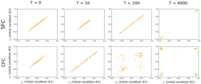
The image presents a 2x4 matrix of scatter plots. Each plot displays the relationship between `x₁` (initial condition #1) and `x₂` (initial condition #2). The plots are arranged to show the evolution of this relationship over time, with time points `T = 0`, `T = 10`, `T = 100`, and `T = 4000`. The top row represents the "SFC" (likely a system or model abbreviation), and the bottom row represents "CFC". The plots show how the initial conditions evolve over time for both SFC and CFC.
### Components/Axes
* **X-axis (all plots):** `x₁` (initial condition #1), ranging from approximately -0.10 to 0.10.
* **Y-axis (all plots):** `x₂` (initial condition #2), ranging from approximately -0.05 to 0.05.
* **Titles (above each plot):** Indicate the time point `T` at which the scatter plot is generated: `T = 0`, `T = 10`, `T = 100`, `T = 4000`.
* **Row Labels (left side):** Indicate the system being analyzed: "SFC" (top row) and "CFC" (bottom row).
* **Data Points:** Orange colored scatter points.
### Detailed Analysis or Content Details
**SFC Plots:**
* **T = 0:** The points form a nearly perfect, positive linear correlation. Approximately 50 points are visible. `x₁` ranges from -0.08 to 0.08, and `x₂` ranges from -0.03 to 0.03.
* **T = 10:** The points continue to show a strong positive linear correlation, very similar to T=0. Approximately 50 points are visible. `x₁` ranges from -0.08 to 0.08, and `x₂` ranges from -0.03 to 0.03.
* **T = 100:** The points still exhibit a strong positive linear correlation, but with slightly more scatter than at T=0 and T=10. Approximately 50 points are visible. `x₁` ranges from -0.08 to 0.08, and `x₂` ranges from -0.03 to 0.03.
* **T = 4000:** The points are now significantly scattered, no longer forming a clear linear relationship. Approximately 100 points are visible. `x₁` ranges from -0.10 to 0.10, and `x₂` ranges from -0.05 to 0.05.
**CFC Plots:**
* **T = 0:** The points form a nearly perfect, positive linear correlation, similar to the SFC plot at T=0. Approximately 50 points are visible. `x₁` ranges from -0.08 to 0.08, and `x₂` ranges from -0.03 to 0.03.
* **T = 10:** The points continue to show a strong positive linear correlation, very similar to T=0. Approximately 50 points are visible. `x₁` ranges from -0.08 to 0.08, and `x₂` ranges from -0.03 to 0.03.
* **T = 100:** The points begin to show some scatter, but still maintain a generally positive correlation. Approximately 50 points are visible. `x₁` ranges from -0.08 to 0.08, and `x₂` ranges from -0.03 to 0.03.
* **T = 4000:** The points are highly scattered, with no discernible linear relationship. Approximately 100 points are visible. `x₁` ranges from -0.10 to 0.10, and `x₂` ranges from -0.05 to 0.05.
### Key Observations
* Both SFC and CFC initially exhibit a strong, positive linear correlation between `x₁` and `x₂`.
* As time progresses, the correlation weakens.
* At `T = 4000`, both SFC and CFC show a completely randomized distribution of points, indicating a loss of predictability or a transition to chaotic behavior.
* The scatter in the SFC plots appears to increase more gradually than in the CFC plots.
### Interpretation
The data suggests that both the SFC and CFC systems start from a predictable state (strong correlation at T=0) but diverge over time. The increasing scatter in the plots indicates a loss of determinism and a potential transition to chaotic behavior. The fact that both systems eventually become completely randomized at T=4000 suggests a common underlying dynamic or sensitivity to initial conditions. The difference in the rate of divergence between SFC and CFC could indicate different sensitivities to perturbations or different underlying mechanisms driving the evolution of the system. The initial linear relationship suggests a simple, predictable relationship between the initial conditions, but the subsequent divergence implies that the systems are more complex and influenced by factors not captured by the initial conditions alone. This could be a visualization of Lyapunov exponents, where the divergence rate is related to the exponent.