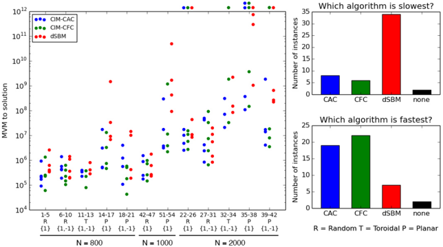
## Scatter Plot & Bar Charts: Algorithm Performance Comparison ### Overview The image presents a comparison of three algorithms – CIM-CAC, CIM-CFC, and dSBM – across different graph types (Random, Toroidal, Planar) and sizes (N=800, N=1000, N=2000). The left side displays a scatter plot showing the number of MVM (Multiplication-Vector Multiplication) operations to solution for each algorithm and instance. The right side contains two bar charts: one indicating which algorithm is slowest, and the other indicating which algorithm is fastest. ### Components/Axes * **Left Plot:** * **X-axis:** Instance labels, combining graph type (R=Random, T=Toroidal, P=Planar) and a numerical identifier (1-5, 6-10, etc.). The N value (800, 1000, 2000) is indicated below the x-axis. * **Y-axis:** Number of MVM to solution, on a logarithmic scale from 10⁴ to 10¹². * **Legend (Top-Left):** * Blue circles: CIM-CAC * Green triangles: CIM-CFC * Red circles: dSBM * **Right Plots:** * **X-axis:** Algorithm names: CAC, CFC, dSBM, none. * **Y-axis:** Number of instances (0-35). * **Top Bar Chart Title:** "Which algorithm is slowest?" * **Bottom Bar Chart Title:** "Which algorithm is fastest?" * **Legend (Bottom-Right):** R = Random, Toroidal, P = Planar. This legend applies to the instance labels on the left plot. ### Detailed Analysis or Content Details **Left Plot (Scatter Plot):** * **CIM-CAC (Blue):** Generally clusters in the lower range of MVM counts (10⁵ - 10⁸) for N=800 and N=1000. For N=2000, the points are more dispersed, ranging from approximately 2x10⁵ to 8x10⁸. * **CIM-CFC (Green):** Shows a wider spread than CIM-CAC. For N=800, values range from approximately 1x10⁵ to 3x10⁷. For N=1000, the range is approximately 1x10⁵ to 5x10⁷. For N=2000, the range expands to approximately 1x10⁵ to 1x10⁹. * **dSBM (Red):** Consistently exhibits the highest MVM counts. For N=800, values range from approximately 2x10⁶ to 2x10⁸. For N=1000, the range is approximately 2x10⁶ to 2x10⁹. For N=2000, the range is approximately 2x10⁶ to 3x10¹⁰. **Right Plots (Bar Charts):** * **Which algorithm is slowest?** * CAC: Approximately 8 instances. * CFC: Approximately 6 instances. * dSBM: Approximately 32 instances. * none: Approximately 2 instances. * **Which algorithm is fastest?** * CAC: Approximately 10 instances. * CFC: Approximately 22 instances. * dSBM: Approximately 8 instances. * none: Approximately 2 instances. ### Key Observations * dSBM consistently requires the most MVM operations to reach a solution, and is identified as the slowest algorithm in the majority of instances. * CIM-CFC is frequently the fastest algorithm, as indicated by the bar chart. * As the graph size (N) increases, the MVM counts generally increase for all algorithms, but the increase is most pronounced for dSBM. * The "none" category in the bar charts suggests that in some instances, no algorithm was able to find a solution within a reasonable number of MVM operations. ### Interpretation The data suggests that CIM-CFC is the most efficient algorithm for solving these types of problems, particularly as the graph size increases. dSBM, while potentially capable of finding a solution, is significantly more computationally expensive. CIM-CAC falls between the two in terms of performance. The logarithmic scale on the Y-axis of the scatter plot highlights the substantial differences in computational cost between the algorithms. The fact that dSBM consistently requires orders of magnitude more MVM operations than the other algorithms suggests that it may be unsuitable for large graphs. The presence of the "none" category in the bar charts indicates that some instances are particularly challenging and may require alternative approaches or more powerful computational resources. The graph type (Random, Toroidal, Planar) also appears to influence performance, as evidenced by the varying distribution of points within each category on the scatter plot. Further analysis would be needed to determine the specific characteristics of each graph type that contribute to these differences.