\n
## Table: Iterative Optimization Steps
### Overview
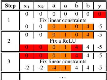
The image presents a table detailing iterative steps in an optimization process, likely related to neural network training or a similar machine learning context. The table tracks the values of variables (x1, x2, â, a, b̂, b) and the output (y) across each step. Color-coding highlights changes in variable values.
### Components/Axes
The table has the following columns:
* **Step:** Integer representing the iteration number (1, 2, 3, and ellipsis indicating continuation).
* **x1:** Numerical value.
* **x2:** Numerical value.
* **â:** Numerical value.
* **a:** Numerical value.
* **b̂:** Numerical value.
* **b:** Numerical value.
* **y:** Numerical value representing the output.
Each row represents a step in the iterative process. Text annotations describe the action taken in each step ("Fix linear constraints", "Fix a ReLU").
### Detailed Analysis or Content Details
Here's a breakdown of the data in each step:
**Step 1:**
* x1 = 0
* x2 = 0
* â = 0
* a = 0
* b̂ = 0
* b = 0
* y = 0 (highlighted in red)
* Action: "Fix linear constraints"
* x1 = 0
* x2 = 0
* â = 0
* a = 1
* b̂ = 0
* b = 4
* y = -5
**Step 2:**
* x1 = 0
* x2 = 0
* â = 0
* a = 1
* b̂ = 0
* b = 4
* y = -5
* Action: "Fix a ReLU"
* x1 = 0
* x2 = 0
* â = 0
* a = 1
* b̂ = 4
* b = 4
* y = -5
**Step 3:**
* x1 = 0
* x2 = 0
* â = 0
* a = 1
* b̂ = 4
* b = 4
* y = -5
* Action: "Fix linear constraints"
* x1 = -2
* x2 = -2
* â = -4
* a = 1
* b̂ = 4
* b = 4
* y = -5
The ellipsis (...) indicates that the process continues beyond step 3.
### Key Observations
* The values of x1, x2, and â become negative in step 3, while a, b̂, and b remain non-negative.
* The output 'y' remains constant at -5 throughout the observed steps.
* The color-coding clearly shows which variables are being modified in each step. Red indicates a change from the previous value within that step. Orange indicates a value that has been fixed in that step.
* The actions alternate between "Fix linear constraints" and "Fix a ReLU", suggesting an iterative optimization algorithm that alternates between enforcing linear constraints and applying a ReLU activation function.
### Interpretation
This table likely represents a simplified illustration of an optimization algorithm used in training a neural network with ReLU activation functions. The algorithm appears to be attempting to minimize some loss function (implied by the 'y' value) by iteratively adjusting the values of the variables x1, x2, â, a, b̂, and b.
The alternating steps of "Fix linear constraints" and "Fix a ReLU" suggest a coordinate descent or similar optimization strategy. The ReLU function introduces non-linearity, and the algorithm is likely trying to find values for the variables that satisfy both the linear constraints and the ReLU activation function while minimizing the output 'y'.
The constant value of 'y' (-5) throughout the observed steps could indicate that the algorithm is still in the early stages of optimization and has not yet converged to a minimum, or that the loss function is flat in the current region of the parameter space. The negative values appearing in step 3 suggest the algorithm is exploring regions of the parameter space where some variables may need to be negative to achieve a better solution. The table provides a visual representation of how the algorithm iteratively refines the variable values to approach an optimal solution.