## Table: Optimization Process with Constraints and Activation Function
### Overview
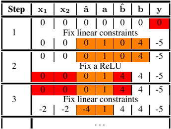
The image depicts a step-by-step optimization process involving linear constraints and a ReLU (Rectified Linear Unit) activation function. The table tracks variables (`x1`, `x2`, `â`, `a`, `b̂`, `b`, `y`) across three steps, with highlighted values indicating parameter adjustments. Text annotations describe operations applied at each stage.
### Components/Axes
- **Columns**:
- `x1`, `x2`: Input variables (fixed at 0 in all steps).
- `â`, `a`: Parameters for linear constraints (highlighted in orange).
- `b̂`, `b`: Parameters for ReLU activation (highlighted in orange).
- `y`: Output value (highlighted in red).
- **Rows**:
- Step 1: Initial state with all zeros except `y=0` (red).
- Step 2: After applying ReLU activation.
- Step 3: After applying linear constraints again.
- **Annotations**:
- "Fix linear constraints" (Step 1 and 3).
- "Fix a ReLU" (Step 2).
### Detailed Analysis
1. **Step 1**:
- `x1=0`, `x2=0`, `â=0`, `a=0`, `b̂=0`, `b=0`, `y=0` (red).
- Annotation: "Fix linear constraints" (applied to `â`, `a`, `b̂`, `b`).
2. **Step 2**:
- `â=0`, `a=1`, `b̂=0`, `b=4` (orange highlights).
- `y=-5` (unchanged from Step 1).
- Annotation: "Fix a ReLU" (applied to `a` and `b`).
3. **Step 3**:
- `â=-2`, `a=1`, `b̂=-4`, `b=4` (orange highlights).
- `y=-5` (unchanged from Step 2).
- Annotation: "Fix linear constraints" (applied to `â`, `a`, `b̂`, `b`).
### Key Observations
- **Parameter Adjustments**:
- `a` transitions from `0` (Step 1) to `1` (Step 2/3), indicating activation of the linear constraint.
- `b` increases from `0` to `4` (Step 2) and remains fixed (Step 3).
- `â` and `b̂` shift to negative values (`-2`, `-4`) in Step 3, suggesting adjustments to satisfy constraints.
- **Output Stability**: `y` remains `-5` after Step 2, implying convergence or a fixed point in the optimization.
- **Color Coding**: Red highlights (`y`) denote critical output values, while orange highlights (`â`, `a`, `b̂`, `b`) indicate adjustable parameters.
### Interpretation
This table illustrates an iterative optimization process where linear constraints and ReLU activation are applied to adjust parameters (`â`, `a`, `b̂`, `b`) to achieve a target output (`y`). The red highlights on `y` emphasize its role as the objective function, while orange highlights show parameters modified at each step. The ReLU activation (`a=1`, `b=4`) introduces non-linearity, while subsequent linear constraints (`â=-2`, `b̂=-4`) refine the solution. The stable `y=-5` suggests the process stabilizes after Step 2, with further adjustments in Step 3 fine-tuning parameters without altering the output. The use of ReLU and linear constraints indicates a hybrid approach to balancing non-linearity and optimization efficiency.