# Technical Document Extraction: Model Control Analysis
This document provides a comprehensive extraction of the data and trends presented in the provided image, which contains three distinct plots labeled **a** and **b**.
---
## Section 1: Component Isolation
The image is divided into two primary segments:
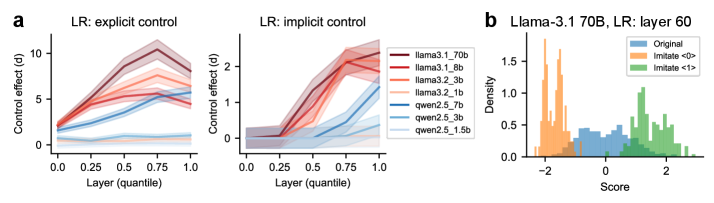
- **Segment A (Left and Center):** Two line graphs comparing "explicit control" and "implicit control" across various LLM architectures.
- **Segment B (Right):** A density histogram showing score distributions for a specific model (Llama-3.1 70B) at a specific layer.
---
## Section 2: Segment A - Control Effect Analysis
### 1. Metadata and Axis Definitions
* **Y-Axis (Both Plots):** "Control effect (d)". This represents the magnitude of the control influence.
* **X-Axis (Both Plots):** "Layer (quantile)". Values range from 0.0 to 1.0, representing the relative depth within the neural network layers.
* **Legend (Shared, located at [x=0.55, y=0.5] relative to Segment A):**
* **Llama Series (Red/Brown hues):**
* `llama3.1_70b` (Darkest Brown)
* `llama3.1_8b` (Dark Red)
* `llama3.2_3b` (Medium Orange-Red)
* `llama3.2_1b` (Light Peach)
* **Qwen Series (Blue hues):**
* `qwen2.5_7b` (Dark Blue)
* `qwen2.5_3b` (Medium Blue)
* `qwen2.5_1.5b` (Light Blue)
### 2. Plot A (Left): LR: explicit control
**Trend Verification:** Most models show a "hump" or "bell" shaped trend. The control effect increases as layers progress toward the middle-late stages (0.75 quantile) before tapering off slightly at the final layers.
* **Key Data Observations:**
* **llama3.1_70b:** Shows the strongest effect, peaking at ~10.5 (d) at the 0.75 layer quantile.
* **llama3.1_8b & llama3.2_3b:** Follow a similar trajectory, peaking between 5.0 and 7.5 (d).
* **qwen2.5_7b:** Shows a steady upward slope, reaching ~5.5 (d) at the 0.75 quantile.
* **Smaller models (llama3.2_1b, qwen2.5_3b, qwen2.5_1.5b):** Exhibit significantly lower control effects, remaining relatively flat near the 0-1 (d) range across all layers.
### 3. Plot A (Center): LR: implicit control
**Trend Verification:** Unlike explicit control, implicit control remains near zero for the first 25% of layers (0.0 to 0.25 quantile) and then exhibits a sharp upward slope for larger models.
* **Key Data Observations:**
* **llama3.1_70b & llama3.1_8b:** Both show a sharp increase after the 0.25 quantile, reaching a plateau or peak between 2.0 and 2.5 (d) at the 0.75-1.0 quantile.
* **qwen2.5_7b:** Shows a delayed but steady increase starting after the 0.5 quantile, reaching ~1.5 (d) at the final layer.
* **Smallest models:** The lines for `llama3.2_1b` and `qwen2.5_1.5b` remain essentially flat at 0 (d) throughout all layers, indicating negligible implicit control.
---
## Section 3: Segment B - Score Density Distribution
### 1. Metadata and Axis Definitions
* **Title:** "b Llama-3.1 70B, LR: layer 60"
* **Y-Axis:** "Density" (Scale: 0.0 to 1.5+)
* **X-Axis:** "Score" (Scale: -2 to 2)
* **Legend (Located at [x=0.85, y=0.8]):**
* **Original (Blue):** Baseline distribution.
* **Imitate <0> (Orange):** Distribution shifted toward negative scores.
* **Imitate <1> (Green):** Distribution shifted toward positive scores.
### 2. Data Distribution and Trends
* **Original (Blue):** A broad, relatively flat distribution centered around 0. It spans roughly from -1.5 to +1.5.
* **Imitate <0> (Orange):** A high-density, narrow peak (bimodal) concentrated between -2.5 and -1.0. The highest peak reaches a density of approximately 1.8 at score -2.0.
* **Imitate <1> (Green):** A high-density distribution concentrated between 0.5 and 2.5. The primary peak is centered around score 1.2 with a density of approximately 1.1.
**Conclusion for Segment B:** The "Imitate" interventions successfully shift the model's internal score distributions away from the "Original" neutral center toward specific polarities (negative for <0> and positive for <1>).