# Technical Document Extraction: State Transition System
## Overview
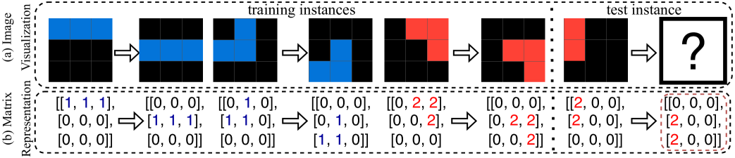
The image depicts a **state transition system** with two primary components:
1. **Visualization** (top section)
2. **Representation** (bottom section)
Both sections illustrate the evolution of a 3x3 grid through training instances and a test instance. The system uses **color-coded states** (blue, red, black) and **numerical matrices** to represent grid configurations.
---
## Visualization Section
### Components
- **Grid Layout**: 3x3 grid with cells colored **blue**, **red**, or **black**.
- **Arrows**: Indicate transitions between states.
- **Question Mark**: Represents an unknown state in the test instance.
### Training Instances (Left to Right)
1. **Initial State**:
- Grid: All cells **blue** (top row) and **black** (bottom two rows).
- Matrix: `[[1,1,1],[0,0,0],[0,0,0]]`
- Legend: Blue = 1, Black = 0
2. **Transition 1**:
- Grid: Middle row **blue**, others **black**.
- Matrix: `[[0,0,0],[1,1,1],[0,0,0]]`
3. **Transition 2**:
- Grid: Top-left and middle-left cells **blue**, others **black**.
- Matrix: `[[0,1,0],[1,1,0],[0,0,0]]`
4. **Transition 3**:
- Grid: Top-left cell **blue**, others **black**.
- Matrix: `[[0,0,0],[0,1,0],[0,0,0]]`
5. **Transition 4**:
- Grid: Top-left and middle-left cells **blue**, others **black**.
- Matrix: `[[0,0,0],[0,1,0],[0,0,0]]`
6. **Transition 5**:
- Grid: Top-left cell **blue**, others **black**.
- Matrix: `[[0,0,0],[0,1,0],[0,0,0]]`
### Test Instance (Rightmost)
- **Grid**: Top-left cell **red**, others **black**.
- **Question Mark**: Indicates an unknown state.
- **Matrix**: `[[2,0,0],[0,0,0],[0,0,0]]`
- **Legend**: Red = 2 (new state introduced in test instance).
---
## Representation Section
### Numerical Matrices
Each grid is mapped to a 3x3 matrix with integer values:
- **0**: Black (background)
- **1**: Blue (initial state)
- **2**: Red (new state in test instance)
### Key Observations
1. **Training Progression**:
- Starts with all **blue** (1s) and **black** (0s).
- Gradually introduces **blue** cells in specific positions.
- Final training instance retains **blue** in the middle-left cell.
2. **Test Instance**:
- Introduces **red** (2) in the top-left cell, a new state not seen in training.
- Matrix: `[[2,0,0],[0,0,0],[0,0,0]]`
---
## Legend and Color Mapping
- **Blue**: Represents value **1** (initial state).
- **Red**: Represents value **2** (new state in test instance).
- **Black**: Represents value **0** (background).
**Legend Placement**: Not explicitly shown in the image, but inferred from color-to-value mapping in matrices.
---
## Spatial Grounding and Trends
### Visual Trends
- **Training Instances**:
- Blue cells (1s) transition from full coverage to sparse distribution.
- No red cells appear in training.
- **Test Instance**:
- Red cell (2) appears in the top-left corner, indicating a novel state.
- All other cells remain **black** (0).
### Component Isolation
1. **Header**: "Visualization" and "Representation" labels.
2. **Main Chart**:
- Training instances (left) → Test instance (right).
- Arrows show state evolution.
3. **Footer**: Numerical matrices and legend (implied).
---
## Data Table Reconstruction
| Instance | Grid State (Visualization) | Matrix Representation (Representation) |
|----------------|-----------------------------------|----------------------------------------------|
| Training 1 | All blue (top), black (bottom) | `[[1,1,1],[0,0,0],[0,0,0]]` |
| Training 2 | Middle row blue | `[[0,0,0],[1,1,1],[0,0,0]]` |
| Training 3 | Top-left and middle-left blue | `[[0,1,0],[1,1,0],[0,0,0]]` |
| Training 4 | Top-left blue | `[[0,0,0],[0,1,0],[0,0,0]]` |
| Training 5 | Top-left blue | `[[0,0,0],[0,1,0],[0,0,0]]` |
| Test Instance | Top-left red, others black | `[[2,0,0],[0,0,0],[0,0,0]]` |
---
## Conclusion
The system demonstrates a **state transition process** where:
1. Training instances evolve from uniform blue states to sparse blue configurations.
2. The test instance introduces a **new red state** (value 2) in the top-left cell, suggesting a prediction or anomaly detection task.
3. Numerical matrices provide a precise representation of grid states, with colors mapped to integers (0=black, 1=blue, 2=red).
This structure enables analysis of state evolution and generalization to unseen configurations.