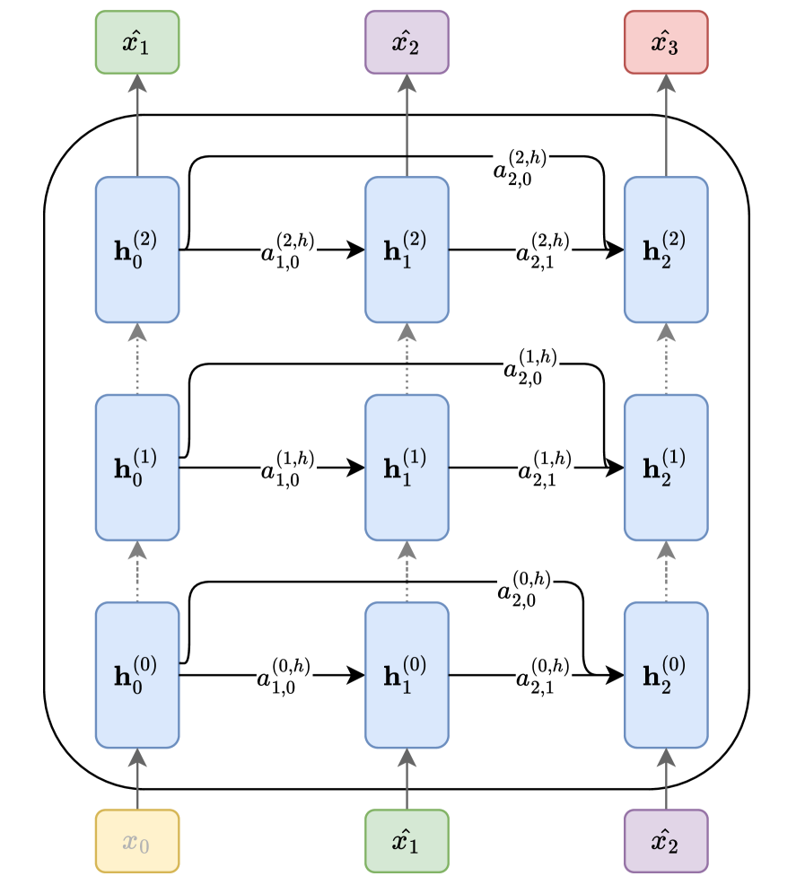
\n ## Diagram: Recurrent Neural Network Unfolding ### Overview The image depicts an unfolded recurrent neural network (RNN) over three time steps. It illustrates the flow of information through the network, showing the connections between input, hidden states, and weights. The diagram highlights the recurrent connections that define the RNN's ability to process sequential data. ### Components/Axes The diagram consists of the following components: * **Input Nodes:** Represented by green rectangles labeled x₀, x₁, x₂, x̂₁, x̂₂, x̂₃. * **Hidden State Nodes:** Represented by blue rounded rectangles labeled h₀⁽⁰⁾, h₁⁽⁰⁾, h₂⁽⁰⁾, h₀⁽¹⁾, h₁⁽¹⁾, h₂⁽¹⁾, h₀⁽²⁾, h₁⁽²⁾, h₂⁽²⁾. The superscript indicates the time step. * **Weight Connections:** Represented by arrows with labels indicating the weight matrix and bias. The labels are in the format a⁽ᵗ⁾, where 't' represents the time step. * **Recurrent Connections:** Represented by curved arrows connecting hidden states across time steps. * **Feedforward Connections:** Represented by straight arrows connecting input nodes to hidden states and hidden states to subsequent hidden states. ### Detailed Analysis The diagram shows three time steps (0, 1, and 2) of an RNN unfolded. Let's analyze the connections and labels: **Time Step 0:** * Input: x₀ connects to h₀⁽⁰⁾, h₁⁽⁰⁾, and h₂⁽⁰⁾. * Weights: a⁽⁰⁾₁₀ connects x₀ to h₀⁽⁰⁾, a⁽⁰⁾₂₁ connects x₀ to h₁⁽⁰⁾, a⁽⁰⁾₂₀ connects x₀ to h₂⁽⁰⁾. **Time Step 1:** * Input: x̂₁ connects to h₀⁽¹⁾, h₁⁽¹⁾, and h₂⁽¹⁾. * Recurrent Connection: h₀⁽⁰⁾ connects to h₀⁽¹⁾, h₁⁽⁰⁾ connects to h₁⁽¹⁾, and h₂⁽⁰⁾ connects to h₂⁽¹⁾. * Weights: a⁽¹⁾₁₀ connects x̂₁ to h₀⁽¹⁾, a⁽¹⁾₂₁ connects x̂₁ to h₁⁽¹⁾, a⁽¹⁾₂₀ connects x̂₁ to h₂⁽¹⁾. a⁽¹⁾₂₀ connects h₀⁽⁰⁾ to h₀⁽¹⁾, a⁽¹⁾₂₁ connects h₁⁽⁰⁾ to h₁⁽¹⁾, a⁽¹⁾₂₀ connects h₂⁽⁰⁾ to h₂⁽¹⁾. **Time Step 2:** * Input: x̂₂ connects to h₀⁽²⁾, h₁⁽²⁾, and h₂⁽²⁾. * Recurrent Connection: h₀⁽¹⁾ connects to h₀⁽²⁾, h₁⁽¹⁾ connects to h₁⁽²⁾, and h₂⁽¹⁾ connects to h₂⁽²⁾. * Weights: a⁽²⁾₁₀ connects x̂₂ to h₀⁽²⁾, a⁽²⁾₂₁ connects x̂₂ to h₁⁽²⁾, a⁽²⁾₂₀ connects x̂₂ to h₂⁽²⁾. a⁽²⁾₂₀ connects h₀⁽¹⁾ to h₀⁽²⁾, a⁽²⁾₂₁ connects h₁⁽¹⁾ to h₁⁽²⁾, a⁽²⁾₂₀ connects h₂⁽¹⁾ to h₂⁽²⁾. Finally, x̂₃ connects to h₀⁽²⁾, h₁⁽²⁾, and h₂⁽²⁾. The weight labels are in the format a⁽ᵗ⁾ᵢⱼ, where: * t is the time step. * i is the index of the hidden unit at the current time step. * j is the index of the hidden unit at the previous time step (for recurrent connections) or the input unit (for feedforward connections). ### Key Observations * The diagram clearly illustrates the recurrent nature of the network, with hidden states at previous time steps influencing the hidden states at subsequent time steps. * The weights (a) are shared across time steps, which is a key characteristic of RNNs. * The diagram shows a fully connected RNN, where each hidden unit receives input from all hidden units at the previous time step and all input units at the current time step. * The input sequence is x₀, x₁, x₂, and the intermediate outputs are x̂₁, x̂₂ and x̂₃. ### Interpretation This diagram demonstrates the core mechanism of an RNN: the ability to maintain a hidden state that captures information about past inputs. The unfolding of the network over time allows us to visualize how the hidden state is updated at each time step based on the current input and the previous hidden state. The shared weights ensure that the network learns to process sequential data in a consistent manner. The diagram is a conceptual representation and doesn't specify the activation functions or the output layer of the RNN. It focuses solely on the flow of information through the recurrent connections and the associated weights. The diagram is a powerful tool for understanding the fundamental principles of RNNs and their ability to model sequential data.