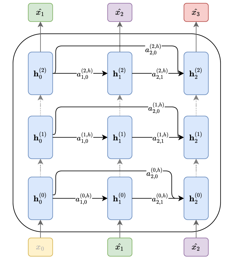
## Diagram: Multi-Layer Recurrent Neural Network with Skip Connections ### Overview The image displays a schematic diagram of a multi-layer recurrent neural network (RNN) architecture. It illustrates the flow of data from input sequences at the bottom, through multiple stacked layers of hidden states, to output sequences at the top. The architecture features both sequential connections within a layer and skip connections that link hidden states across different time steps and layers. ### Components/Axes The diagram is organized into three main vertical sections and multiple horizontal layers. **1. Input Layer (Bottom):** * Three input nodes are positioned at the bottom of the diagram. * From left to right, they are labeled: * `x₀` (in a yellow box) * `x̂₁` (in a green box) * `x̂₂` (in a purple box) **2. Hidden Layers (Middle):** * The core of the diagram consists of three stacked horizontal layers of hidden states, each represented by blue rounded rectangles. * Each layer contains three hidden states, indexed by time step (subscript) and layer (superscript in parentheses). * **Layer 0 (Bottom Hidden Layer):** `h₀⁽⁰⁾`, `h₁⁽⁰⁾`, `h₂⁽⁰⁾` * **Layer 1 (Middle Hidden Layer):** `h₀⁽¹⁾`, `h₁⁽¹⁾`, `h₂⁽¹⁾` * **Layer 2 (Top Hidden Layer):** `h₀⁽²⁾`, `h₁⁽²⁾`, `h₂⁽²⁾` **3. Output Layer (Top):** * Three output nodes are positioned at the top of the diagram. * From left to right, they are labeled: * `x̂₁` (in a green box) * `x̂₂` (in a purple box) * `x̂₃` (in a red box) **4. Connections and Labels:** * **Vertical (Inter-layer) Connections:** Dotted gray arrows point upward from each hidden state `h_t^(l)` to the hidden state at the same time step in the layer above, `h_t^(l+1)`. This represents the flow of information from lower to higher layers. * **Horizontal (Intra-layer) Connections:** Solid black arrows point from a hidden state to the next hidden state within the same layer (e.g., from `h₀⁽⁰⁾` to `h₁⁽⁰⁾`). These are labeled with terms `a`, indicating a learned parameter or gate. * The label format is `a_{destination,source}^{(layer,type)}`. * Example: The connection from `h₀⁽⁰⁾` to `h₁⁽⁰⁾` is labeled `a_{1,0}^{(0,h)}`. * **Skip Connections:** Curved black arrows originate from a hidden state and point to a hidden state at a later time step in the same or a higher layer. These are also labeled with `a` terms. * Example: A connection from `h₀⁽⁰⁾` to `h₂⁽⁰⁾` is labeled `a_{2,0}^{(0,h)}`. * Example: A connection from `h₀⁽¹⁾` to `h₂⁽²⁾` is labeled `a_{2,0}^{(2,h)}`. * **Input to Hidden:** Solid gray arrows point from each input node (`x₀`, `x̂₁`, `x̂₂`) to the corresponding hidden state in the first layer (`h₀⁽⁰⁾`, `h₁⁽⁰⁾`, `h₂⁽⁰⁾`). * **Hidden to Output:** Solid gray arrows point from the top-layer hidden states (`h₀⁽²⁾`, `h₁⁽²⁾`, `h₂⁽²⁾`) to the corresponding output nodes (`x̂₁`, `x̂₂`, `x̂₃`). ### Detailed Analysis The diagram explicitly defines the following connections and their associated parameters (`a` terms): **Layer 0 (l=0):** * `h₀⁽⁰⁾` → `h₁⁽⁰⁾`: `a_{1,0}^{(0,h)}` * `h₁⁽⁰⁾` → `h₂⁽⁰⁾`: `a_{2,1}^{(0,h)}` * `h₀⁽⁰⁾` → `h₂⁽⁰⁾` (skip): `a_{2,0}^{(0,h)}` **Layer 1 (l=1):** * `h₀⁽¹⁾` → `h₁⁽¹⁾`: `a_{1,0}^{(1,h)}` * `h₁⁽¹⁾` → `h₂⁽¹⁾`: `a_{2,1}^{(1,h)}` * `h₀⁽¹⁾` → `h₂⁽¹⁾` (skip): `a_{2,0}^{(1,h)}` **Layer 2 (l=2):** * `h₀⁽²⁾` → `h₁⁽²⁾`: `a_{1,0}^{(2,h)}` * `h₁⁽²⁾` → `h₂⁽²⁾`: `a_{2,1}^{(2,h)}` * `h₀⁽²⁾` → `h₂⁽²⁾` (skip): `a_{2,0}^{(2,h)}` **Cross-Layer Skip Connections:** * `h₀⁽⁰⁾` → `h₂⁽¹⁾`: `a_{2,0}^{(1,h)}` * `h₀⁽¹⁾` → `h₂⁽²⁾`: `a_{2,0}^{(2,h)}` ### Key Observations 1. **Symmetry and Pattern:** The connection pattern is highly regular and repeated across all three layers. Each layer has identical intra-layer connectivity: a forward step to the next time step and a skip connection to the time step two steps ahead. 2. **Parameter Sharing:** The `a` labels suggest that the parameters governing these connections are specific to the destination, source, and layer (e.g., `a_{1,0}^{(0,h)}` is distinct from `a_{1,0}^{(1,h)}`). There is no visual indication of parameter sharing across time steps (like in a standard RNN) or layers. 3. **Input/Output Mapping:** The input sequence (`x₀`, `x̂₁`, `x̂₂`) is mapped to an output sequence (`x̂₁`, `x̂₂`, `x̂₃`) that is shifted by one time step. This is characteristic of sequence prediction tasks (e.g., predicting the next token). 4. **Color Coding:** Inputs and outputs use distinct colors (yellow, green, purple, red), while all hidden states are uniformly blue. This visually separates the external interface from the internal processing units. ### Interpretation This diagram represents a sophisticated **multi-layer recurrent architecture with dense skip connections**. The key insights are: * **Purpose:** The architecture is designed for processing sequential data (like text or time series). The stacked layers allow the network to learn hierarchical representations, with lower layers capturing basic patterns and higher layers capturing more abstract features. * **Flow of Information:** Data flows upward through the layers and forward through time. The **skip connections** (`a_{2,0}` terms) are the most notable feature. They create "shortcuts" that allow information from earlier time steps to directly influence later computations, bypassing intermediate steps. This design helps mitigate the vanishing gradient problem common in deep RNNs, enabling the training of deeper networks and improving the flow of information across long sequences. * **Relationships:** The diagram defines a precise computational graph. The value of any hidden state `h_t^(l)` is a function of: 1. The hidden state from the previous layer at the same time step (`h_t^(l-1)`). 2. The hidden state from the same layer at the previous time step (`h_{t-1}^(l)`). 3. Potentially, hidden states from the same layer at even earlier time steps (via skip connections). * **Anomalies/Notable Features:** The notation `x̂` (x-hat) is used for both some inputs and all outputs, which typically denotes a predicted or estimated value. This suggests the inputs `x̂₁` and `x̂₂` might themselves be predictions from a previous step or part of an auto-regressive setup. The architecture is not a vanilla RNN, LSTM, or GRU but a more generalized form where the specific update rules are parameterized by the various `a` terms, which could represent weights in a linear transformation or gates in a more complex unit.