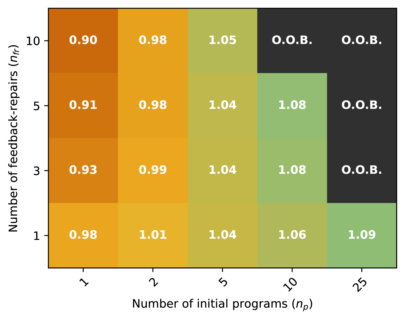
## Heatmap: Performance Metric by Number of Feedback-Repairs and Initial Programs ### Overview This image displays a heatmap illustrating a performance metric across a grid defined by two input parameters: "Number of feedback-repairs" ($n_{fr}$) on the vertical axis and "Number of initial programs" ($n_p$) on the horizontal axis. Each cell in the grid contains a numerical value representing the metric, or the text "O.O.B." (Out Of Bounds), and is colored to visually represent its magnitude. The color gradient transitions from darker orange/brown for lower values, through yellow and light green for increasing values, to darker green for the highest values. Dark grey cells indicate the "O.O.B." state. ### Components/Axes * **Y-axis (Left):** Labeled "Number of feedback-repairs ($n_{fr}$)" * Tick markers (from bottom to top): 1, 3, 5, 10 * **X-axis (Bottom):** Labeled "Number of initial programs ($n_p$)" * Tick markers (from left to right): 1, 2, 5, 10, 25 * **Data Grid:** A 4x5 grid of cells, each containing a numerical value (to two decimal places) or the text "O.O.B.". The background color of each cell visually represents the magnitude of the value. * **Color Gradient (Implicit Legend):** * Darker orange/brown (e.g., 0.90, 0.91, 0.93): Represents lower metric values. * Lighter orange/yellow (e.g., 0.98, 0.99, 1.01): Represents mid-range metric values. * Light green/olive (e.g., 1.04, 1.05, 1.06): Represents higher mid-range metric values. * Darker green (e.g., 1.08, 1.09): Represents the highest metric values. * Dark grey: Represents the "O.O.B." (Out Of Bounds) state. ### Detailed Analysis The heatmap presents the following data, organized by `Number of feedback-repairs` ($n_{fr}$) on the Y-axis and `Number of initial programs` ($n_p$) on the X-axis. | $n_{fr}$ \ $n_p$ | 1 | 2 | 5 | 10 | 25 | | :--------------- | :----- | :----- | :----- | :----- | :----- | | **10** | 0.90 | 0.98 | 1.05 | O.O.B. | O.O.B. | | **5** | 0.91 | 0.98 | 1.04 | 1.08 | O.O.B. | | **3** | 0.93 | 0.99 | 1.04 | 1.08 | O.O.B. | | **1** | 0.98 | 1.01 | 1.04 | 1.06 | 1.09 | **Trends:** * **Across rows (increasing $n_p$ for a fixed $n_{fr}$):** * For $n_{fr}=10$: The metric values increase from 0.90 (dark orange) to 0.98 (yellow) to 1.05 (light green), then transition to "O.O.B." (dark grey) for $n_p=10$ and $n_p=25$. * For $n_{fr}=5$: The metric values increase from 0.91 (dark orange) to 0.98 (yellow) to 1.04 (light green) to 1.08 (dark green), then become "O.O.B." (dark grey) for $n_p=25$. * For $n_{fr}=3$: The metric values increase from 0.93 (dark orange) to 0.99 (yellow) to 1.04 (light green) to 1.08 (dark green), then become "O.O.B." (dark grey) for $n_p=25$. * For $n_{fr}=1$: The metric values consistently increase from 0.98 (yellow) to 1.01 (yellow) to 1.04 (light green) to 1.06 (light green) to 1.09 (dark green). * General trend: As the "Number of initial programs" ($n_p$) increases, the performance metric generally improves (increases), until it reaches an "O.O.B." state for higher $n_p$ values, particularly when $n_{fr}$ is also high. * **Down columns (increasing $n_{fr}$ for a fixed $n_p$):** * For $n_p=1$: The metric values decrease from 0.98 (yellow) to 0.93 (dark orange) to 0.91 (dark orange) to 0.90 (dark orange). * For $n_p=2$: The metric values decrease from 1.01 (yellow) to 0.99 (yellow) to 0.98 (yellow) and remain stable at 0.98 (yellow). * For $n_p=5$: The metric values are relatively stable at 1.04 (light green) for $n_{fr}=1, 3, 5$, then slightly increase to 1.05 (light green) for $n_{fr}=10$. * For $n_p=10$: The metric values increase from 1.06 (light green) to 1.08 (dark green) for $n_{fr}=3, 5$, then become "O.O.B." (dark grey) for $n_{fr}=10$. * For $n_p=25$: The metric value is 1.09 (dark green) for $n_{fr}=1$, then becomes "O.O.B." (dark grey) for $n_{fr}=3, 5, 10$. * General trend: The impact of increasing "Number of feedback-repairs" ($n_{fr}$) varies. For lower $n_p$, the metric tends to decrease or stabilize. For higher $n_p$, the metric tends to increase before hitting "O.O.B." for the highest $n_{fr}$ values. ### Key Observations * The lowest observed metric value is 0.90, located at the top-left corner ($n_{fr}=10, n_p=1$). * The highest observed metric value is 1.09, located at the bottom-right corner of the non-O.O.B. region ($n_{fr}=1, n_p=25$). * The "O.O.B." state appears in the upper-right portion of the heatmap, indicating that for higher values of $n_p$ (10 and 25) combined with higher values of $n_{fr}$ (3, 5, 10), the system enters an "Out Of Bounds" condition. * There is a clear diagonal boundary for the "O.O.B." region, starting from ($n_{fr}=10, n_p=10$) and extending downwards and rightwards to include ($n_{fr}=3, n_p=25$), ($n_{fr}=5, n_p=25$), and ($n_{fr}=10, n_p=25$). * The performance metric generally improves as $n_p$ increases, but this improvement is limited by the onset of the "O.O.B." state. * For $n_p=1$, increasing $n_{fr}$ consistently decreases the metric. For $n_p=2$, increasing $n_{fr}$ leads to a slight decrease and then stabilization. For $n_p=5$, the metric is relatively stable. For $n_p=10$ and $n_p=25$, increasing $n_{fr}$ initially improves the metric but quickly leads to "O.O.B.". ### Interpretation This heatmap likely illustrates the performance characteristics of a system or algorithm influenced by two parameters: the number of feedback-repairs ($n_{fr}$) and the number of initial programs ($n_p$). Higher metric values are generally associated with better performance, as indicated by the color progression from orange (low) to green (high). The data suggests that increasing the "Number of initial programs" ($n_p$) is generally beneficial for performance, leading to higher metric values. This trend is most pronounced when the "Number of feedback-repairs" ($n_{fr}$) is low (e.g., $n_{fr}=1$), where the metric continuously increases to its peak of 1.09. However, there's a critical interaction with $n_{fr}$. While increasing $n_p$ is good, combining high $n_p$ with high $n_{fr}$ leads to an "Out Of Bounds" (O.O.B.) state. This "O.O.B." condition could signify system failure, instability, resource exhaustion, or a state where the metric cannot be meaningfully computed. The diagonal boundary of the O.O.B. region indicates a threshold or limit where the combined complexity or resource demands of many initial programs and many feedback-repairs become unmanageable. Conversely, the effect of increasing $n_{fr}$ is not uniformly positive. For a small number of initial programs ($n_p=1, 2$), more feedback-repairs actually lead to slightly worse or stable performance. For moderate $n_p$ (e.g., $n_p=5$), $n_{fr}$ has little impact on the metric. Only when $n_p$ is already high (e.g., $n_p=10$) does increasing $n_{fr}$ initially boost performance before quickly pushing the system into the O.O.B. state. In summary, the system achieves its best measurable performance (1.09) with a high number of initial programs ($n_p=25$) and a low number of feedback-repairs ($n_{fr}=1$). This suggests an optimal operating point where the system benefits from a broad initial exploration (many initial programs) but is sensitive to excessive iterative refinement or correction (feedback-repairs), especially when the initial exploration is already extensive. The "O.O.B." region highlights a critical operational boundary that must be avoided for stable and measurable system behavior.