\n
## Scatter Plot: Relationship of Space Size and Gap Ratio
### Overview
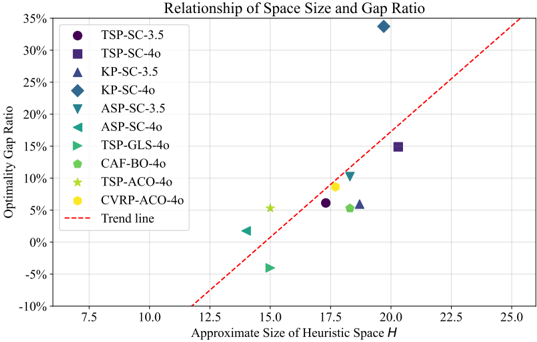
This image presents a scatter plot illustrating the relationship between the "Approximate Size of Heuristic Space H" (x-axis) and the "Optimality Gap Ratio" (y-axis). Multiple data series, each representing a different algorithm or problem instance, are plotted as distinct markers. A trend line is also included.
### Components/Axes
* **Title:** Relationship of Space Size and Gap Ratio
* **X-axis:** Approximate Size of Heuristic Space H (Scale: 7.5 to 25.0, increments of 2.5)
* **Y-axis:** Optimality Gap Ratio (Scale: -10% to 35%, increments of 5%)
* **Legend:** Located in the top-left corner, listing the following data series with corresponding marker shapes and colors:
* TSP-SC-3.5 (Purple Circle)
* TSP-SC-4o (Purple Square)
* KP-SC-3.5 (Blue Triangle)
* KP-SC-4o (Blue Diamond)
* ASP-SC-3.5 (Green Triangle)
* ASP-SC-4o (Green Square)
* TSP-GLS-4o (Olive Green Triangle)
* CAF-BO-4o (Olive Green Circle)
* TSP-ACO-4o (Yellow Star)
* CVRP-ACO-4o (Yellow Circle)
* **Trend Line:** Dashed red line, extending diagonally across the plot.
### Detailed Analysis
The data points are scattered across the plot, with varying degrees of correlation to the trend line. Here's a breakdown of each data series, with approximate values based on visual inspection:
* **TSP-SC-3.5 (Purple Circle):** The line slopes upward. Data points are approximately (15.5, -2%), (17.5, 6%), (19.0, 15%).
* **TSP-SC-4o (Purple Square):** The line is relatively flat. Data point is approximately (20.0, 15%).
* **KP-SC-3.5 (Blue Triangle):** The line slopes upward. Data point is approximately (17.5, 25%).
* **KP-SC-4o (Blue Diamond):** The line slopes downward. Data point is approximately (20.0, 32%).
* **ASP-SC-3.5 (Green Triangle):** The line slopes upward. Data point is approximately (15.0, 2%).
* **ASP-SC-4o (Green Square):** The line slopes upward. Data point is approximately (17.5, 10%).
* **TSP-GLS-4o (Olive Green Triangle):** The line slopes upward. Data point is approximately (15.0, -5%).
* **CAF-BO-4o (Olive Green Circle):** The line slopes upward. Data point is approximately (18.0, 8%).
* **TSP-ACO-4o (Yellow Star):** The line slopes upward. Data point is approximately (17.5, 5%).
* **CVRP-ACO-4o (Yellow Circle):** The line slopes upward. Data point is approximately (15.5, 3%).
The trend line itself appears to approximate a 45-degree angle, suggesting a positive correlation between the Approximate Size of Heuristic Space H and the Optimality Gap Ratio.
### Key Observations
* The data points are widely dispersed, indicating a weak to moderate correlation overall.
* KP-SC-4o (Blue Diamond) has the highest Optimality Gap Ratio, at approximately 32%, and a relatively high Approximate Size of Heuristic Space H, around 20.
* TSP-GLS-4o (Olive Green Triangle) has a negative Optimality Gap Ratio, approximately -5%, and a relatively low Approximate Size of Heuristic Space H, around 15.
* The trend line does not perfectly fit all data points, with some points lying significantly above or below it.
### Interpretation
The plot explores the trade-off between the size of the search space (Approximate Size of Heuristic Space H) and the quality of the solution found (Optimality Gap Ratio). A larger search space *could* lead to better solutions (lower gap ratio), but it also increases the computational cost. The trend line suggests that, on average, increasing the search space tends to improve solution quality, but the scatter of the data indicates that this relationship is not deterministic.
The significant variation among the different algorithms (TSP-SC, KP-SC, ASP-SC, etc.) suggests that the effectiveness of increasing the search space depends heavily on the specific algorithm used. Some algorithms (like TSP-GLS-4o) appear to achieve good results even with a relatively small search space, while others (like KP-SC-4o) require a larger space to achieve comparable performance.
The outlier data points (e.g., TSP-GLS-4o with a negative gap ratio) may indicate cases where the algorithm has found a solution that is actually *better* than the optimal solution, or that the optimality gap calculation is flawed. Further investigation would be needed to determine the cause of these anomalies. The data suggests that there is no single "best" approach, and the optimal strategy depends on the specific problem and the available computational resources.