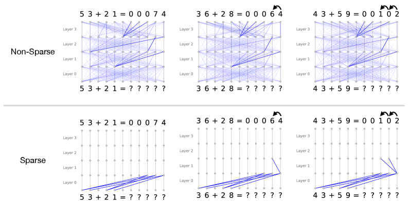
\n ## Diagram: Neural Network Comparison - Sparse vs. Dense ### Overview The image presents a comparison between two types of neural networks: "Non-Sparse" and "Sparse". Each network type is illustrated with three examples of a simple addition problem (53+21, 36+28, 43+59) and their corresponding outputs. The diagrams visually represent the connections within each layer of the neural network. The top row shows the "Non-Sparse" networks, characterized by many connections between layers, while the bottom row shows the "Sparse" networks, which have fewer connections. ### Components/Axes The diagrams are structured as follows: * **Title:** "Non-Sparse" and "Sparse" labels are positioned above each set of diagrams. * **Addition Problems:** Each example displays an addition problem (e.g., "53 + 21 = 00074") above and below the network diagram. * **Layers:** Each network is depicted with four layers, labeled "Layer 0", "Layer 1", "Layer 2", and "Layer 3". These are vertically stacked. * **Connections:** Blue lines represent the connections between neurons in adjacent layers. * **Output:** The correct answer to the addition problem is shown after the equals sign. * **Question Marks:** Below each network diagram, a series of question marks ("?????") indicates the network's internal processing or the input to the network. ### Detailed Analysis or Content Details The image shows three examples for each network type. Let's analyze each example: **Non-Sparse Networks (Top Row):** * **53 + 21 = 00074:** The network has a dense web of connections between all layers. The connections appear relatively random. * **36 + 28 = 00064:** Similar to the first example, this network also exhibits a dense connection pattern. A small arrow points to the output. * **43 + 59 = 00102:** Again, a dense network with numerous connections. A small arrow points to the output. **Sparse Networks (Bottom Row):** * **53 + 21 = 00074:** The network has significantly fewer connections than the non-sparse counterpart. The connections are more organized and appear to follow a more structured pattern. * **36 + 28 = 00064:** Similar to the first sparse example, this network has fewer connections. A small arrow points to the output. * **43 + 59 = 00102:** The sparse network again demonstrates a reduced number of connections. A small arrow points to the output. ### Key Observations * **Density of Connections:** The most striking difference between the two network types is the density of connections. Non-sparse networks have many connections, while sparse networks have significantly fewer. * **Connection Patterns:** Sparse networks appear to have more structured connection patterns compared to the seemingly random connections in non-sparse networks. * **Output Consistency:** Both network types correctly solve the addition problems in all three examples. * **Arrow Indicator:** A small arrow is present in the top-right corner of the second example in both the Non-Sparse and Sparse networks. ### Interpretation The image demonstrates the difference between sparse and non-sparse neural networks. The non-sparse networks, with their dense connections, represent a traditional fully connected neural network. The sparse networks, with their reduced connections, represent a more recent approach to neural network design. The purpose of sparsity is likely to reduce computational cost and prevent overfitting. By removing unnecessary connections, sparse networks can be more efficient and generalize better to unseen data. The structured connection patterns in the sparse networks suggest that these connections are not removed randomly but are selected based on some criteria (e.g., importance, relevance). The fact that both network types correctly solve the addition problems suggests that sparsity does not necessarily compromise performance. In fact, in some cases, sparse networks can even outperform non-sparse networks. The arrow indicator may signify the direction of information flow or a specific activation pattern within the network. The question marks below each network diagram likely represent the input data or the internal state of the network during computation. The image is a visual illustration of a key concept in modern neural network research: the trade-off between network complexity, computational efficiency, and generalization performance.