## Line Graphs: E_train vs. c for Different K and r Values
### Overview
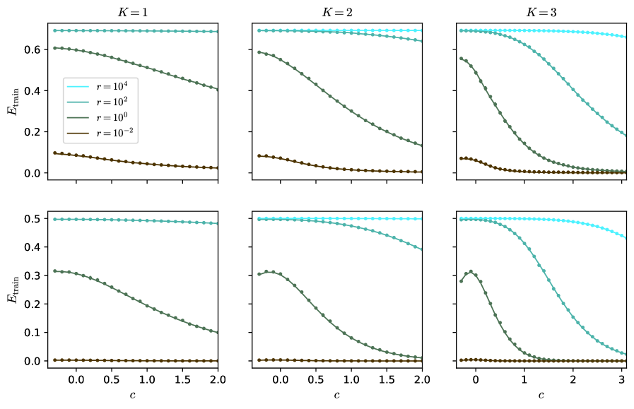
The image contains six line graphs arranged in a 2x3 grid, each representing the relationship between the training error (`E_train`) and a parameter `c` for different values of `K` (1, 2, 3) and `r` (10⁴, 10², 10⁰, 10⁻²). The graphs show how `E_train` evolves as `c` increases, with distinct trends for each combination of `K` and `r`.
---
### Components/Axes
- **X-axis (c)**: Ranges from 0 to 3 in all graphs. Labeled as `c`.
- **Y-axis (E_train)**: Ranges from 0 to 0.6 in the top row and 0 to 0.5 in the bottom row. Labeled as `E_train`.
- **Legend**: Located in the top-left corner of the entire figure. Colors correspond to:
- `r = 10⁴`: Light blue (dashed line)
- `r = 10²`: Teal (dotted line)
- `r = 10⁰`: Dark green (solid line)
- `r = 10⁻²`: Brown (dotted line)
- **Grid Layout**:
- Top row: `K = 1`, `K = 2`, `K = 3`
- Bottom row: `K = 1`, `K = 2`, `K = 3` (same as top row but with different y-axis scaling)
---
### Detailed Analysis
#### **K = 1**
- **Light blue (r = 10⁴)**: Flat line at ~0.6, indicating no change in `E_train` as `c` increases.
- **Teal (r = 10²)**: Slightly declining trend, starting near 0.6 and dropping to ~0.4 by `c = 2`.
- **Dark green (r = 10⁰)**: Steeper decline, starting at ~0.6 and falling to ~0.2 by `c = 2`.
- **Brown (r = 10⁻²)**: Gradual decline from ~0.1 to ~0.05 over `c = 0` to `c = 2`.
#### **K = 2**
- **Light blue (r = 10⁴)**: Flat line at ~0.6.
- **Teal (r = 10²)**: Declines from ~0.6 to ~0.4 by `c = 2`.
- **Dark green (r = 10⁰)**: Steeper drop from ~0.6 to ~0.2 by `c = 2`.
- **Brown (r = 10⁻²)**: Minimal change, hovering near 0.05.
#### **K = 3**
- **Light blue (r = 10⁴)**: Flat line at ~0.6.
- **Teal (r = 10²)**: Declines from ~0.6 to ~0.3 by `c = 3`.
- **Dark green (r = 10⁰)**: Sharp drop from ~0.6 to ~0.1 by `c = 2`, then stabilizes.
- **Brown (r = 10⁻²)**: Remains near 0.05 throughout.
#### **Bottom Row (K = 1, 2, 3)**
- **Y-axis scaled to 0–0.5** (vs. 0–0.6 in the top row).
- **Trends mirror the top row** but with compressed `E_train` values:
- For `K = 1`, `r = 10⁰` drops to ~0.1 by `c = 2`.
- For `K = 3`, `r = 10⁰` drops to ~0.05 by `c = 2`.
---
### Key Observations
1. **Inverse Relationship Between `r` and `E_train`**:
- Higher `r` values (e.g., 10⁴, 10²) maintain higher `E_train` and show minimal sensitivity to `c`.
- Lower `r` values (e.g., 10⁻²) result in lower `E_train` and sharper declines as `c` increases.
2. **Impact of `K`**:
- Higher `K` values amplify the effect of `r` on `E_train`. For example:
- At `K = 3`, `r = 10⁰` drops to ~0.1 (top row) vs. ~0.2 (bottom row).
- At `K = 1`, `r = 10⁰` drops to ~0.2 (top row) vs. ~0.1 (bottom row).
3. **Stability of `r = 10⁴`**:
- The light blue line (`r = 10⁴`) remains flat across all `K` values, suggesting it acts as a stabilizing parameter.
4. **Consistency of `r = 10⁻²`**:
- The brown line (`r = 10⁻²`) is consistently the lowest across all graphs, indicating minimal training error regardless of `c` or `K`.
---
### Interpretation
The data suggests that `r` acts as a regularization parameter, where higher values (e.g., 10⁴) suppress overfitting (maintaining higher `E_train`), while lower values (e.g., 10⁻²) allow the model to adapt more closely to the training data (lower `E_train`). The parameter `K` likely represents model complexity (e.g., number of layers or components), with higher `K` values exacerbating the sensitivity of `E_train` to `r`. For instance:
- At `K = 3`, even moderate `r` values (e.g., 10⁰) lead to significant drops in `E_train` as `c` increases, implying overfitting in complex models.
- The flat `r = 10⁴` line across all `K` values indicates it may represent a baseline or theoretical upper limit for training error.
This pattern is critical for tuning hyperparameters in machine learning models, where balancing `r` and `K` is essential to avoid overfitting while maintaining model performance.