\n
## Directed Graph Diagram: Hierarchical Network Structure
### Overview
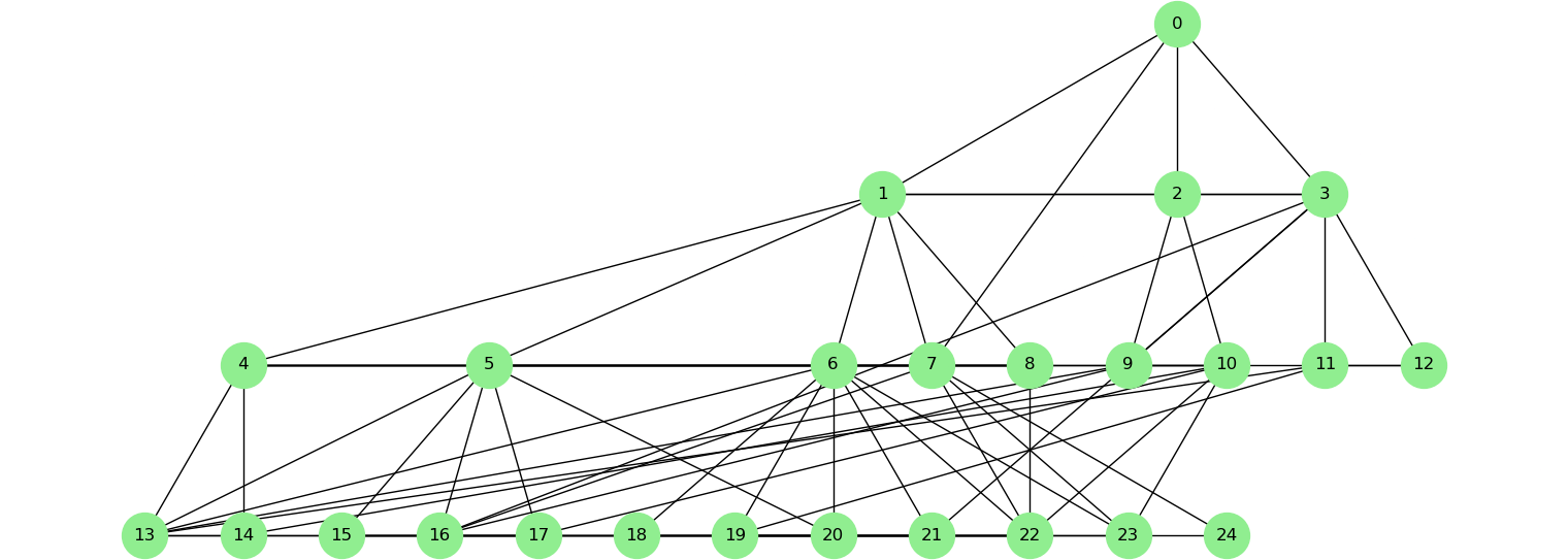
The image displays a directed graph (or network diagram) consisting of 25 nodes, labeled with integers from 0 to 24. The nodes are arranged in a hierarchical, layered structure with directed edges (lines) connecting them, indicating a flow or relationship from higher to lower layers. The graph appears to represent a multi-level network, such as an organizational chart, a data flow diagram, or a dependency tree.
### Components/Axes
* **Nodes:** 25 circular nodes, each filled with a light green color and containing a unique integer label (0 through 24).
* **Edges:** Directed lines (black) connecting nodes, indicating a one-way relationship or flow from a source node to a target node.
* **Layout:** The graph is organized into four distinct horizontal layers or tiers.
* **Layer 0 (Top):** Contains a single node: **0**.
* **Layer 1:** Contains three nodes: **1, 2, 3**.
* **Layer 2:** Contains nine nodes: **4, 5, 6, 7, 8, 9, 10, 11, 12**.
* **Layer 3 (Bottom):** Contains twelve nodes: **13, 14, 15, 16, 17, 18, 19, 20, 21, 22, 23, 24**.
### Detailed Analysis
**Node Connectivity and Flow:**
The flow is strictly top-down. Connections exist between adjacent layers, with no visible connections within the same layer or skipping layers.
1. **From Layer 0 (Node 0):**
* Node 0 has directed edges to all three nodes in Layer 1: **1, 2, and 3**.
2. **From Layer 1:**
* **Node 1** connects to nodes **4, 5, 6, 7, 8, 9, 10, 11** in Layer 2.
* **Node 2** connects to nodes **6, 7, 8, 9, 10, 11** in Layer 2.
* **Node 3** connects to nodes **9, 10, 11, 12** in Layer 2.
3. **From Layer 2:**
* **Node 4** connects to nodes **13, 14** in Layer 3.
* **Node 5** connects to nodes **13, 14, 15, 16, 17, 18** in Layer 3.
* **Node 6** connects to nodes **13, 14, 15, 16, 17, 18, 19, 20** in Layer 3.
* **Node 7** connects to nodes **13, 14, 15, 16, 17, 18, 19, 20, 21** in Layer 3.
* **Node 8** connects to nodes **13, 14, 15, 16, 17, 18, 19, 20, 21, 22** in Layer 3.
* **Node 9** connects to nodes **13, 14, 15, 16, 17, 18, 19, 20, 21, 22, 23** in Layer 3.
* **Node 10** connects to nodes **13, 14, 15, 16, 17, 18, 19, 20, 21, 22, 23, 24** in Layer 3.
* **Node 11** connects to nodes **13, 14, 15, 16, 17, 18, 19, 20, 21, 22, 23, 24** in Layer 3.
* **Node 12** connects to nodes **23, 24** in Layer 3.
**Spatial Grounding:**
* **Node 0** is positioned at the top-center of the diagram.
* **Layer 1 (Nodes 1, 2, 3)** is positioned directly below Node 0, spaced evenly across the width.
* **Layer 2 (Nodes 4-12)** is positioned below Layer 1, with nodes spread across the full width. Nodes 4 and 5 are on the far left, nodes 11 and 12 are on the far right.
* **Layer 3 (Nodes 13-24)** forms the bottom row, spanning the entire width of the diagram.
* The density of connecting lines increases significantly from the top layer to the bottom layer, creating a complex web in the lower half of the diagram.
### Key Observations
1. **Increasing Fan-Out:** The number of outgoing connections (fan-out) from nodes generally increases as you move down the hierarchy. Node 0 has a fan-out of 3, Layer 1 nodes have fan-outs ranging from 4 to 8, and Layer 2 nodes have fan-outs ranging from 2 to 12.
2. **Central Hub Nodes:** Nodes **6, 7, 8, 9, 10, and 11** in Layer 2 act as major hubs, receiving connections from multiple Layer 1 nodes and distributing connections to nearly all nodes in Layer 3.
3. **Peripheral Nodes:** Nodes **4, 5, and 12** in Layer 2 have more limited connectivity, linking to specific subsets of the bottom layer. Node 12, in particular, only connects to the last two nodes (23, 24).
4. **Complete Connectivity in Lower Layers:** The bottom layer (Nodes 13-24) is highly interconnected from above. Most nodes in Layer 3 receive connections from multiple sources in Layer 2, suggesting a many-to-many relationship or a robust distribution network at the base.
### Interpretation
This diagram represents a **hierarchical broadcast or distribution network**. The structure suggests a system where information, commands, or resources flow from a single source (Node 0) through intermediate distributors (Layers 1 and 2) to a broad base of end-points (Layer 3).
* **Function:** It could model an organizational command structure, a computer network topology, a supply chain, or a data dissemination protocol.
* **Robustness & Redundancy:** The high connectivity in the lower layers implies redundancy. If a hub node in Layer 2 fails, its target nodes in Layer 3 likely still receive input from other hub nodes, making the system resilient.
* **Bottleneck Potential:** Nodes in Layer 1 and the central hubs in Layer 2 are critical points. Failure of Node 0 or Node 1, for example, would disrupt flow to a large portion of the network.
* **Scalability:** The design is scalable at the bottom (Layer 3 can be expanded) but may face bottlenecks at the middle layers if the number of end-points grows significantly without adding more intermediate distributors.
**Note:** The diagram contains no textual labels beyond the node identifiers (0-24). There are no axis titles, legends, or data values to extract, as this is a structural diagram, not a data chart. The primary information is the topology itself—the nodes and their directed connections.