\n
## Diagram: Causal Structures & Information Flow
### Overview
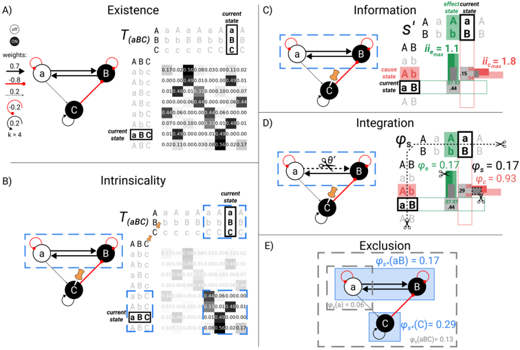
The image presents five distinct diagrams (A-E) illustrating different causal structures and information flow concepts. Each diagram features a network of nodes (a, b, c) connected by directed edges, accompanied by a matrix representing the transition probabilities between states. The diagrams are labeled "Existence", "Intrinsicality", "Information", "Integration", and "Exclusion". Each diagram also includes a small matrix representing the effect/current state.
### Components/Axes
Each diagram shares the following components:
* **Nodes:** Represented by circles labeled 'a', 'b', and 'c'.
* **Directed Edges:** Arrows indicating the direction of causal influence. Edge weights are indicated numerically.
* **Transition Matrix (T(ABC)):** A 4x4 matrix representing the probabilities of transitioning between states ABC, Abc, aBC, and abc. Rows and columns are labeled with these states.
* **Effect/Current State Matrix:** A 2x2 matrix representing the effect/current state.
* **Labels:** Each diagram has a title indicating the concept it illustrates.
* **Color Coding:** Red indicates activation/influence, while black indicates no influence.
### Detailed Analysis or Content Details
**A) Existence**
* **Edge Weights:** a->b: 0.2, b->c: 0.2, c->a: -0.2.
* **Transition Matrix T(ABC):**
* ABC: 0.11, 0.02, 0.03, 0.02
* Abc: 0.00, 0.45, 0.10, 0.00
* aBC: 0.00, 0.00, 0.60, 0.00
* abc: 0.00, 0.00, 0.00, 0.50
* **Current State:** aBC (highlighted in blue).
* **Effect/Current State Matrix:** S' = 1.1, ii<sub>c</sub> = 1.8
**B) Intrinsicality**
* **Edge Weights:** a->b: 0.2, b->c: 0.2, c->a: -0.2. (Same as A)
* **Transition Matrix T(ABC):** (Identical to A)
* ABC: 0.11, 0.02, 0.03, 0.02
* Abc: 0.00, 0.45, 0.10, 0.00
* aBC: 0.00, 0.00, 0.60, 0.00
* abc: 0.00, 0.00, 0.00, 0.50
* **Current State:** abc (highlighted in blue).
* **Effect/Current State Matrix:** S' = 0.6, ii<sub>c</sub> = 0.6
**C) Information**
* **Edge Weights:** a->b: (red), b->c: (red), a->c: (red).
* **Transition Matrix:** Not fully visible, but shows values like 0.71, 0.44.
* **Current State:** Ab (highlighted in blue).
* **Effect/Current State Matrix:** ii<sub>max</sub> = 1.1, ii<sub>c</sub> = 1.8
**D) Integration**
* **Edge Weights:** a->b: (red), b->c: (red), c->a: (red). Angle θ' is indicated.
* **Φ<sub>s</sub>:** 0.17
* **Φ<sub>c</sub>:** 0.93
* **Transition Matrix:** Not fully visible, but shows values like 97.61.
* **Current State:** aB (highlighted in blue).
**E) Exclusion**
* **Edge Weights:** a->b: (red), b->c: (red).
* **Φ<sub>s</sub>(aB):** 0.17
* **Φ<sub>c</sub>(a):** 0.06
* **Φ<sub>c</sub>(a,b):** 0.29
* **Φ<sub>c</sub>(a,b,c):** 0.13
* **Transition Matrix:** Not fully visible.
* **Current State:** ab (highlighted in blue).
### Key Observations
* Diagrams A and B share the same network structure and transition matrix, differing only in the highlighted current state.
* The "Information" diagram (C) shows all nodes influencing each other.
* The "Integration" diagram (D) introduces an angle θ' and uses Φ values (likely representing some form of correlation or influence strength).
* The "Exclusion" diagram (E) introduces multiple Φ values, suggesting a more complex relationship between the nodes.
* The matrices are not fully visible, making precise data extraction difficult.
### Interpretation
These diagrams appear to be exploring different types of causal relationships within a simple three-node system. The transition matrices quantify the probabilities of the system being in different states, while the edge weights represent the strength of causal influence.
* **Existence & Intrinsicality (A & B):** These diagrams demonstrate how the same underlying causal structure can lead to different system states. The difference in current state (aBC vs. abc) highlights the sensitivity to initial conditions.
* **Information (C):** This diagram suggests a fully connected system where information can flow freely between all nodes.
* **Integration (D):** The introduction of the angle θ' and Φ values suggests a more nuanced relationship, potentially representing the degree of integration or synergy between the nodes. The high Φ<sub>c</sub> value (0.93) indicates a strong correlation in the current state.
* **Exclusion (E):** The multiple Φ values in this diagram suggest that the influence of one node on another is contingent on the state of other nodes. The lower Φ<sub>c</sub>(a) value (0.06) suggests that node 'a' has a limited influence on the system when considered in isolation.
The diagrams collectively illustrate how different causal structures and information flow patterns can emerge within a simple system, and how these patterns can be quantified using probabilistic models. The use of color coding (red for activation, black for no influence) provides a visual representation of the causal relationships. The matrices provide a quantitative measure of the system's dynamics. The diagrams are likely part of a larger theoretical framework exploring the foundations of information processing and causality.