\n ## Diagram: Mathematical Solution Process Annotation ### Overview The image is a technical diagram illustrating two methods of annotating and evaluating the solution process for a specific mathematical problem. It contrasts a simple outcome-based annotation with a more granular process-based annotation, using a concrete example to demonstrate how different solution paths can lead to correct or incorrect final answers. ### Components/Axes The diagram is organized into several distinct regions: 1. 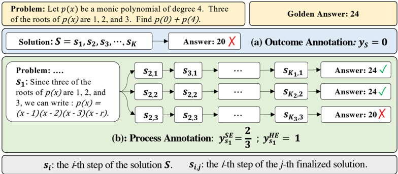**Header Region (Top):** * **Problem Statement (Top-Left):** "Problem: Let \( p(x) \) be a monic polynomial of degree 4. Three of the roots of \( p(x) \) are 1, 2, and 3. Find \( p(0) + p(4) \)." * **Golden Answer (Top-Right):** "Golden Answer: 24" 2. **Main Process Region (Center):** * **Part (a) Outcome Annotation:** A single horizontal flow. * Input: "Solution: \( S = s_1, s_2, s_3, \cdots, s_K \)" * Process: An arrow points to a box containing "Answer: 20 ❌". * Annotation Label: "(a) Outcome Annotation: \( y_S = 0 \)" * **Part (b) Process Annotation:** A branching flow showing multiple solution attempts. * **Root Problem Box (Left):** "Problem: ...." * **First Step Box (\( s_1 \)):** "\( s_1 \); Since three of the roots of \( p(x) \) are 1, 2, and 3, we can write: \( p(x) = (x-1)(x-2)(x-3)(x-r) \)." * **Branching Paths:** Three parallel horizontal flows originate from the \( s_1 \) box, labeled for \( j = 1, 2, 3 \). * **Path j=1 (Top):** \( s_{2,1} \rightarrow s_{3,1} \rightarrow \cdots \rightarrow s_{K,1} \) leading to "Answer: 24 ✅". * **Path j=2 (Middle):** \( s_{2,2} \rightarrow s_{3,2} \rightarrow \cdots \rightarrow s_{K,2} \) leading to "Answer: 24 ✅". * **Path j=3 (Bottom):** \( s_{2,3} \rightarrow s_{3,3} \rightarrow \cdots \rightarrow s_{K,3} \) leading to "Answer: 20 ❌". * **Annotation Label:** "(b): Process Annotation: \( y_{s_1}^{SE} = \frac{2}{3} \) ; \( y_{s_1}^{HE} = 1 \)" 3. **Footer/Legend Region (Bottom):** * **Legend:** "\( s_i \): the \( i \)-th step of the solution \( S \). \( s_{i,j} \): the \( i \)-th step of the \( j \)-th finalized solution." ### Detailed Analysis * **Problem & Solution:** The core problem involves finding the value of \( p(0) + p(4) \) for a monic quartic polynomial with known roots 1, 2, and 3. The "Golden Answer" is established as 24. * **Outcome Annotation (a):** This evaluates the entire solution process \( S \) as a single unit. The final answer derived is 20, which is incorrect (marked with ❌). The annotation \( y_S = 0 \) likely represents a binary score (0 for incorrect, 1 for correct). * **Process Annotation (b):** This evaluates the first critical step \( s_1 \) of the solution. The step \( s_1 \) correctly sets up the polynomial form \( p(x) = (x-1)(x-2)(x-3)(x-r) \). From this single correct starting point, three distinct "finalized solutions" (j=1,2,3) are shown. * Two of these paths (j=1 and j=2) lead to the correct answer of 24 (✅). * One path (j=3) leads to the incorrect answer of 20 (❌). * **Process Metrics:** Two metrics are derived from this branching: * \( y_{s_1}^{SE} = \frac{2}{3} \): This appears to be a "Success Efficiency" or similar metric, calculated as the ratio of correct final answers (2) to total attempted paths (3) stemming from step \( s_1 \). * \( y_{s_1}^{HE} = 1 \): This likely represents a "Human Efficiency" or "Heuristic Efficiency" score, possibly indicating that the initial step \( s_1 \) itself is fundamentally correct or optimal, regardless of subsequent errors in some paths. ### Key Observations 1. **Divergence from a Common Start:** All three solution paths share the identical, correct first step (\( s_1 \)). The divergence into correct and incorrect outcomes must therefore occur in the subsequent steps (\( s_{2,j} \) onwards). 2. **Annotation Granularity:** The diagram highlights the difference between evaluating only the final output (Outcome Annotation) versus evaluating the quality of a pivotal intermediate step (Process Annotation). 3. **Visual Coding:** Correct answers are consistently marked with green checkmarks (✅) and incorrect ones with red crosses (❌). The branching structure in part (b) is visually clear, with arrows indicating the flow of reasoning. ### Interpretation This diagram serves as a conceptual model for evaluating problem-solving processes, particularly in educational or AI training contexts. It argues that judging a solution solely by its final answer (Outcome Annotation) can be misleading. A student or an AI model might start with a perfectly valid strategy (step \( s_1 \)) but make an error later, resulting in a wrong answer. The Process Annotation method focuses on the quality of that critical initial step. The metrics \( y_{s_1}^{SE} \) and \( y_{s_1}^{HE} \) suggest a framework for quantifying the robustness or reliability of a given solution step. A step that leads to a correct answer 2 out of 3 times (\( SE = 2/3 \)) might be considered good but not foolproof, while a step that is fundamentally sound (\( HE = 1 \)) is valuable even if some execution paths fail. The diagram implies that for effective learning or model training, feedback should be directed at these pivotal decision points (like \( s_1 \)) rather than just the final outcome. It visually advocates for a more nuanced, process-oriented assessment of mathematical reasoning.