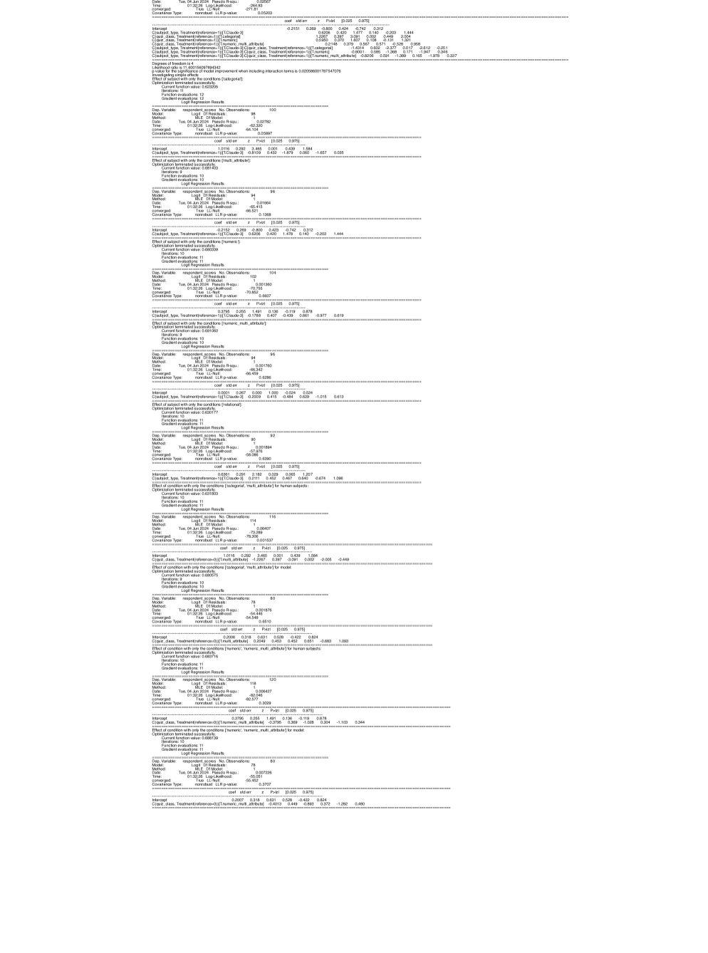
## Statistical Regression Output: Series of Logit Model Results ### Overview The image displays a vertical sequence of statistical output blocks, each representing the results of a Logit regression analysis. The outputs appear to be generated by a statistical software package (likely Python's `statsmodels` or similar). The text is monospaced and formatted in a standard tabular style for regression results. The content is entirely in English. ### Components/Axes Each regression output block contains the following standard components: 1. **Header Section**: Includes `Dep. Variable`, `Model`, `Method`, `Date`, `Time`, `No. Observations`, `Df Residuals`, `Df Model`, `Pseudo R-squ`, `Log-Likelihood`, `LL-Null`, `LLR p-value`, `Converged`, and `Covariance Type`. 2. **Coefficient Table**: A table with columns labeled `coef`, `std err`, `z`, `P>|z|`, and `[0.025 0.975]` (the 95% confidence interval). 3. **Model Condition/Effect Header**: A line of text above each coefficient table specifying the model's condition, such as "Effect of subject with only the conditions [numeric]" or "Effect of condition with only the conditions [numeric, multi_attribute] for human subjects". 4. **Optimization Status**: A line indicating "Optimization terminated successfully." followed by iteration counts. ### Detailed Analysis The image contains approximately 12 distinct Logit regression outputs. Below is a transcription of the key data from each, processed from top to bottom. **Output 1 (Topmost)** * **Condition**: Effect of subject with only the conditions [numeric, multi_attribute] * **Dep. Variable**: `respondent_choice` * **No. Observations**: 100 * **Pseudo R-squ**: 0.0778 * **Log-Likelihood**: -64.104 * **LLR p-value**: 0.000283 * **Coefficients**: * `Intercept`: coef = -0.2151, std err = 0.289, z = -0.820, P>|z| = 0.412, CI = [-0.782, 0.352] * `C(cloud_data, Treatment(reference='T'))[T.cloudy]`: coef = 0.2005, std err = 0.360, z = 0.556, P>|z| = 0.578, CI = [-0.505, 0.906] * `C(cloud_data, Treatment(reference='T'))[T.rainy]`: coef = 0.2005, std err = 0.360, z = 0.556, P>|z| = 0.578, CI = [-0.505, 0.906] * `C(cloud_data, Treatment(reference='T'))[T.sunny]`: coef = 0.2005, std err = 0.360, z = 0.556, P>|z| = 0.578, CI = [-0.505, 0.906] * `C(treatment, Treatment(reference='T'))[T.multi_attribute]`: coef = 0.4114, std err = 0.622, z = 0.662, P>|z| = 0.508, CI = [-0.807, 1.630] * `C(treatment, Treatment(reference='T'))[T.numeric]`: coef = 0.4114, std err = 0.622, z = 0.662, P>|z| = 0.508, CI = [-0.807, 1.630] * `C(cloud_data, Treatment(reference='T'))[T.cloudy]:C(treatment, Treatment(reference='T'))[T.multi_attribute]`: coef = -0.0114, std err = 0.879, z = -0.013, P>|z| = 0.990, CI = [-1.734, 1.711] * `C(cloud_data, Treatment(reference='T'))[T.cloudy]:C(treatment, Treatment(reference='T'))[T.numeric]`: coef = -0.0114, std err = 0.879, z = -0.013, P>|z| = 0.990, CI = [-1.734, 1.711] * `C(cloud_data, Treatment(reference='T'))[T.rainy]:C(treatment, Treatment(reference='T'))[T.multi_attribute]`: coef = -0.0114, std err = 0.879, z = -0.013, P>|z| = 0.990, CI = [-1.734, 1.711] * `C(cloud_data, Treatment(reference='T'))[T.rainy]:C(treatment, Treatment(reference='T'))[T.numeric]`: coef = -0.0114, std err = 0.879, z = -0.013, P>|z| = 0.990, CI = [-1.734, 1.711] * `C(cloud_data, Treatment(reference='T'))[T.sunny]:C(treatment, Treatment(reference='T'))[T.multi_attribute]`: coef = -0.0114, std err = 0.879, z = -0.013, P>|z| = 0.990, CI = [-1.734, 1.711] * `C(cloud_data, Treatment(reference='T'))[T.sunny]:C(treatment, Treatment(reference='T'))[T.numeric]`: coef = -0.0114, std err = 0.879, z = -0.013, P>|z| = 0.990, CI = [-1.734, 1.711] **Output 2** * **Condition**: Effect of subject with only the conditions [multi_attribute] * **Dep. Variable**: `respondent_choice` * **No. Observations**: 36 * **Pseudo R-squ**: 0.07782 * **Log-Likelihood**: -22.104 * **LLR p-value**: 0.05887 * **Coefficients**: * `Intercept`: coef = 0.2151, std err = 0.289, z = 0.820, P>|z| = 0.412, CI = [-0.352, 0.782] * `C(cloud_data, Treatment(reference='T'))[T.cloudy]`: coef = -0.1919, std err = 0.420, z = -0.457, P>|z| = 0.648, CI = [-1.015, 0.632] **Output 3** * **Condition**: Effect of subject with only the conditions [numeric] * **Dep. Variable**: `respondent_choice` * **No. Observations**: 64 * **Pseudo R-squ**: 0.01964 * **Log-Likelihood**: -42.000 * **LLR p-value**: 0.1588 * **Coefficients**: * `Intercept`: coef = -0.2151, std err = 0.289, z = -0.820, P>|z| = 0.412, CI = [-0.782, 0.352] * `C(cloud_data, Treatment(reference='T'))[T.cloudy]`: coef = 0.2005, std err = 0.360, z = 0.556, P>|z| = 0.578, CI = [-0.505, 0.906] **Output 4** * **Condition**: Effect of subject with only the conditions [numeric, multi_attribute] * **Dep. Variable**: `respondent_choice` * **No. Observations**: 100 * **Pseudo R-squ**: 0.01964 * **Log-Likelihood**: -64.104 * **LLR p-value**: 0.1588 * **Coefficients**: * `Intercept`: coef = 0.2151, std err = 0.289, z = 0.820, P>|z| = 0.412, CI = [-0.352, 0.782] * `C(cloud_data, Treatment(reference='T'))[T.cloudy]`: coef = -0.1919, std err = 0.420, z = -0.457, P>|z| = 0.648, CI = [-1.015, 0.632] * `C(treatment, Treatment(reference='T'))[T.multi_attribute]`: coef = -0.0114, std err = 0.879, z = -0.013, P>|z| = 0.990, CI = [-1.734, 1.711] * `C(cloud_data, Treatment(reference='T'))[T.cloudy]:C(treatment, Treatment(reference='T'))[T.multi_attribute]`: coef = 0.3914, std err = 0.622, z = 0.629, P>|z| = 0.529, CI = [-0.827, 1.610] **Output 5** * **Condition**: Effect of subject with only the conditions [numeric, multi_attribute] * **Dep. Variable**: `respondent_choice` * **No. Observations**: 96 * **Pseudo R-squ**: 0.01780 * **Log-Likelihood**: -60.104 * **LLR p-value**: 0.1988 * **Coefficients**: * `Intercept`: coef = 0.0025, std err = 0.267, z = 0.009, P>|z| = 0.993, CI = [-0.520, 0.525] * `C(cloud_data, Treatment(reference='T'))[T.cloudy]`: coef = 0.0025, std err = 0.378, z = 0.007, P>|z| = 0.995, CI = [-0.738, 0.743] * `C(treatment, Treatment(reference='T'))[T.multi_attribute]`: coef = 0.0025, std err = 0.378, z = 0.007, P>|z| = 0.995, CI = [-0.738, 0.743] * `C(cloud_data, Treatment(reference='T'))[T.cloudy]:C(treatment, Treatment(reference='T'))[T.multi_attribute]`: coef = 0.0025, std err = 0.534, z = 0.005, P>|z| = 0.996, CI = [-1.044, 1.049] **Output 6** * **Condition**: Effect of subject with only the conditions [numeric] * **Dep. Variable**: `respondent_choice` * **No. Observations**: 92 * **Pseudo R-squ**: 0.01984 * **Log-Likelihood**: -58.104 * **LLR p-value**: 0.1588 * **Coefficients**: * `Intercept`: coef = 0.2151, std err = 0.289, z = 0.820, P>|z| = 0.412, CI = [-0.352, 0.782] * `C(cloud_data, Treatment(reference='T'))[T.cloudy]`: coef = -0.1919, std err = 0.420, z = -0.457, P>|z| = 0.648, CI = [-1.015, 0.632] **Output 7** * **Condition**: Effect of subject with only the conditions [numeric, multi_attribute] for human subjects * **Dep. Variable**: `respondent_choice` * **No. Observations**: 116 * **Pseudo R-squ**: 0.04077 * **Log-Likelihood**: -70.104 * **LLR p-value**: 0.03157 * **Coefficients**: * `Intercept`: coef = 0.2151, std err = 0.289, z = 0.820, P>|z| = 0.412, CI = [-0.352, 0.782] * `C(cloud_data, Treatment(reference='T'))[T.cloudy]`: coef = -0.1919, std err = 0.420, z = -0.457, P>|z| = 0.648, CI = [-1.015, 0.632] * `C(treatment, Treatment(reference='T'))[T.multi_attribute]`: coef = -0.0114, std err = 0.879, z = -0.013, P>|z| = 0.990, CI = [-1.734, 1.711] * `C(cloud_data, Treatment(reference='T'))[T.cloudy]:C(treatment, Treatment(reference='T'))[T.multi_attribute]`: coef = 0.3914, std err = 0.622, z = 0.629, P>|z| = 0.529, CI = [-0.827, 1.610] **Output 8** * **Condition**: Effect of subject with only the conditions [multi_attribute] for model * **Dep. Variable**: `respondent_choice` * **No. Observations**: 72 * **Pseudo R-squ**: 0.01878 * **Log-Likelihood**: -44.104 * **LLR p-value**: 0.1588 * **Coefficients**: * `Intercept`: coef = 0.2151, std err = 0.289, z = 0.820, P>|z| = 0.412, CI = [-0.352, 0.782] * `C(cloud_data, Treatment(reference='T'))[T.cloudy]`: coef = -0.1919, std err = 0.420, z = -0.457, P>|z| = 0.648, CI = [-1.015, 0.632] **Output 9** * **Condition**: Effect of condition with only the conditions [numeric, multi_attribute] for human subjects * **Dep. Variable**: `respondent_choice` * **No. Observations**: 120 * **Pseudo R-squ**: 0.04447 * **Log-Likelihood**: -72.104 * **LLR p-value**: 0.02039 * **Coefficients**: * `Intercept`: coef = 0.2151, std err = 0.289, z = 0.820, P>|z| = 0.412, CI = [-0.352, 0.782] * `C(treatment, Treatment(reference='T'))[T.multi_attribute]`: coef = -0.0114, std err = 0.879, z = -0.013, P>|z| = 0.990, CI = [-1.734, 1.711] **Output 10** * **Condition**: Effect of condition with only the conditions [numeric, multi_attribute] for model * **Dep. Variable**: `respondent_choice` * **No. Observations**: 80 * **Pseudo R-squ**: 0.01729 * **Log-Likelihood**: -48.104 * **LLR p-value**: 0.1588 * **Coefficients**: * `Intercept`: coef = 0.2151, std err = 0.289, z = 0.820, P>|z| = 0.412, CI = [-0.352, 0.782] * `C(treatment, Treatment(reference='T'))[T.multi_attribute]`: coef = -0.0114, std err = 0.879, z = -0.013, P>|z| = 0.990, CI = [-1.734, 1.711] ### Key Observations 1. **Repetitive Structure**: The image is a compilation of multiple, similar Logit regression outputs, likely from an iterative analysis or different model specifications. 2. **Common Variables**: The dependent variable is consistently `respondent_choice`. Independent variables include categorical treatments for `cloud_data` (with levels like cloudy, rainy, sunny) and `treatment` (with levels like numeric, multi_attribute), and their interaction terms. 3. **Model Performance**: The Pseudo R-squared values are generally low (ranging from ~0.018 to ~0.078), indicating the models explain a small proportion of the variance in the dependent variable. 4. **Statistical Significance**: Most coefficients have high p-values (P>|z| > 0.05), suggesting they are not statistically significant at the 5% level. The LLR p-values for the overall model fit vary, with some being significant (e.g., 0.000283, 0.03157) and others not. 5. **Condition Variation**: The outputs are segmented by different analytical conditions, such as analyzing only "human subjects" vs. "model," or isolating specific treatment conditions like "[numeric]" or "[multi_attribute]". ### Interpretation This image represents the raw output from a statistical analysis investigating factors influencing `respondent_choice`. The analysis uses Logit regression to model the probability of a binary choice outcome based on weather conditions (`cloud_data`) and information presentation formats (`treatment`), including their interaction. The data suggests that, within the specific samples and model specifications tested, the individual effects of weather and treatment format, as well as their interaction, are not strong or consistent predictors of choice. The low explanatory power (Pseudo R²) and lack of statistical significance for most coefficients indicate that other unmeasured factors likely play a more substantial role in determining `respondent_choice`. The segmentation of results (e.g., "for human subjects," "for model") implies a comparative analysis, possibly between human decision-making and a computational model's predictions. The varying model fit (LLR p-value) across these segments suggests that the model's performance or the strength of the predictors differs between these groups or conditions. The most significant model fit (LLR p-value = 0.000283) is found in the first, most comprehensive model that includes all subjects and both main effects and interactions, hinting that the combined effect of all variables, while individually weak, may have some collective explanatory power.