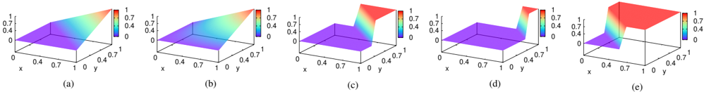
## Surface Plots: Parameter Variation ### Overview The image contains five 3D surface plots, labeled (a) through (e), each depicting a function's output over a 2D input space. The x and y axes range from 0 to 1. The color of the surface represents the function's value, ranging from 0 (blue/purple) to 1 (red), as indicated by the color bar legend. The plots show how the function's behavior changes across the five different parameter settings. ### Components/Axes * **X-axis:** Ranges from 0 to 1, labeled "x". * **Y-axis:** Ranges from 0 to 1, labeled "y". * **Z-axis (Implied):** Represents the function's output value, indicated by the color of the surface. * **Color Bar Legend:** Located to the right of plots (a), (b), and (e). It shows a gradient from blue (value 0) to red (value 1), with intermediate values of 0.4 and 0.7 marked. * **Plot Labels:** (a), (b), (c), (d), and (e) are located below each respective plot. ### Detailed Analysis * **(a):** The surface slopes upward from the bottom-left corner (x=0, y=0) to the top-right corner (x=1, y=1). The color transitions from purple/blue to red, indicating an increasing function value as both x and y increase. The value at (0,0) is approximately 0, and the value at (1,1) is approximately 1. * **(b):** Similar to (a), the surface slopes upward from the bottom-left to the top-right. However, the gradient appears steeper, suggesting a more rapid increase in the function's value. The value at (0,0) is approximately 0, and the value at (1,1) is approximately 1. * **(c):** The surface is mostly flat and purple/blue, indicating a value close to 0. There is a sharp vertical rise along the y=0 axis, where the color changes abruptly to red, indicating a value of 1. The function is approximately 0 for y > 0 and approximately 1 for y = 0. * **(d):** The surface is entirely flat and purple/blue, indicating a constant value of approximately 0 across the entire input space. * **(e):** The surface is mostly flat and purple/blue, indicating a value close to 0. There is a sharp vertical rise along the y=0 axis for x values greater than approximately 0.6, where the color changes abruptly to red, indicating a value of 1. The function is approximately 0 for y > 0 or x < 0.6, and approximately 1 for y = 0 and x > 0.6. ### Key Observations * Plots (a) and (b) show a gradual increase in the function's value with increasing x and y. * Plots (c), (d), and (e) exhibit step-like behavior, with abrupt changes in the function's value. * Plot (d) represents a constant function with a value of 0. * The transition from (a) to (e) shows a shift from a continuous, gradual function to a discontinuous, step-like function. ### Interpretation The image illustrates how different parameter settings can drastically alter the behavior of a function. Plots (a) and (b) might represent a function that is linearly dependent on x and y, while plots (c), (d), and (e) might represent functions with threshold-based behavior. The progression from (a) to (e) suggests a change in the function's parameters that introduces a discontinuity or a sharp threshold. The plots could represent the output of a machine learning model under different training conditions or with different hyperparameter settings. The step-like behavior in (c) and (e) could indicate a decision boundary or a classification rule.